Discontinuous Galerkin (DG) methods form a class of finite element methods particularly suited for solving partial differential equations. Unlike continuous Galerkin methods, DG allows for discontinuities between elements, providing greater flexibility and robustness for complex geometries or highly dynamic phenomena [17] [10] [5].

Pros	Cons
High-order accuracy	Large number of unknowns
Handles non-conforming meshes	Numerous parameters to tune
High arithmetic intensity

A Symmetric Interior Penalty (SIP) method has been implemented in TRUST for solving the Non-Stationary Heat Equation. The SIP method is more performant than mixed DG methods for first- and second-order approximations.

Definitions

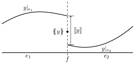
Considering a face \(f\) shared by two cells \(e_1\) and \(e_2\), the interface average of a quantity \(y\):

\[\{\{ y \}\}_f(x) = \frac{1}{2}\left(y|_{e_1}(x) + y|_{e_2}\right) \]

The interface jump (when the normal of \(f\) is defined from \(e_1\) to \(e_2\)):

\[{\left[\!\left[ y \right]\!\right]}_f(x) = y|_{e_1}(x) - y|_{e_2} \]

and otherwise:

\[{\left[\!\left[ y \right]\!\right]}_f(x) = y|_{e_2}(x) - y|_{e_1} \]

Definition of the average and jump notations

SIP DG Method for the Poisson Problem

Find \(u \in H^1_0(\Omega)\) such that:

\[-\text{div}(k\nabla u) = s \quad \Rightarrow \quad a_{dg}(u_h, v_h) = \int_\Omega s\,v_h, \quad \forall v_h \in X_{DG} \]

Discrete bilinear form:

\[\begin{aligned} a_{dg}(u_h, v_h) &= \sum_{e \in E} k_e \int_e \nabla u_h \cdot \nabla v_h \\ &\quad - \sum_{f\in F_e} \int_f k_f \{\{\nabla u_h\}\}_f \cdot \vec{n}_f\,\left[\!\left[v_h\right]\!\right] \\ &\quad - \sum_{f\in F_e} \int_f k_f \{\{\nabla v_h\}\}_f \cdot \vec{n}_f\,\left[\!\left[u_h\right]\!\right] \\ &\quad + \sum_{f\in F_e} \frac{\eta}{h_e} \int_f \left[\!\left[u_h\right]\!\right]_f\,\left[\!\left[v_h\right]\!\right]_f \end{aligned} \]

where \(h_e\) is the diameter of the circumscribed circle of \(e\).

First term: consistency
Second and third terms: symmetry
Last term: stability

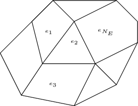
The global stiffness matrix \(\mathbf{K}\) has a block-structured form reflecting the element-wise stencil:

\[\mathbf{K} = \begin{bmatrix} \mathbf{K}_{1,1} & \mathbf{K}_{1,2} & 0 & \cdots \\ \mathbf{K}_{1,2}^e & \mathbf{K}_{2,2} & \mathbf{K}_{2,3} & \cdots \\ 0 & \mathbf{K}_{2,3}^e & \mathbf{K}_{3,3} & \cdots \\ \vdots & & & \ddots \end{bmatrix} \]

Possible mesh with the Discontinuous Galerkin discretization

The stability parameter \(\eta\) is computed automatically to ensure coercivity.

Non-Stationary Heat Equation

For all \(t \in [0, t_{max}]\), find \(T(t) \in H^1_0(\Omega)\) such that:

\[\rho C_p \frac{dT}{dt} - \text{div}(k\nabla T) = s \]

Quantity	Description
\(k\)	Thermal conductivity (W·m⁻¹·K⁻¹)
\(\rho\)	Density (kg·m⁻³)
\(C_p\)	Heat capacity (J·kg⁻¹·K⁻¹)
\(T\)	Temperature (K)
\(s\)	Heat source (W·m⁻³)

Weak form:

\[\rho C_p\,m_{dg}\!\left(\frac{dT_h}{dt},\theta_h\right) + a_{dg}(T_h,\theta_h) = \int_\Omega s\,\theta_h, \quad \forall\theta_h \in X_{DG},\; \forall t\in[0,t_{max}] \]

Time integration:

Implicit Euler: allows larger time steps; requires solving a linear system at each step.
Explicit Euler: fast iterations; requires small time steps (stability constraint).

DG Options

In your data file, add an Option_DG block:

Option_DG
{
    order 2
    gram_schmidt 1
}

order sets the discretization order (only 1 and 2 are currently available). gram_schmidt 1 enables Gram-Schmidt orthonormalization of basis functions, which diagonalizes the mass matrix — useful with explicit schemes.