|
TRUST 1.9.8
HPC thermohydraulic platform
|
|
TRUST 1.9.8
HPC thermohydraulic platform
|
PolyMAC_CDO is based on Compatible Discrete Operator (CDO) schemes [2] [24], designed to apply mimetic finite-volume methods to non-conforming polyhedral meshes with the sole constraint that the cells be star-shaped. In TRUST data files, the keyword PolyMAC is an alias for PolyMAC_CDO.
The major distinction with PolyMAC_MPFA is that vorticity is an explicit unknown of the velocity equation, not a derived quantity, and the viscous term is discretised through a curl–curl decomposition (see "Diffusion operator" below).
Limitation. PolyMAC_CDO does not support multiphase problems (Pb_Multiphase). For multiphase, use PolyMAC_MPFA or PolyMAC_HFV.
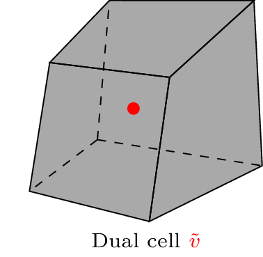
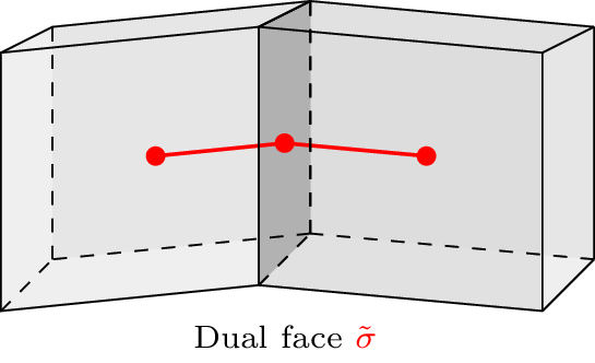
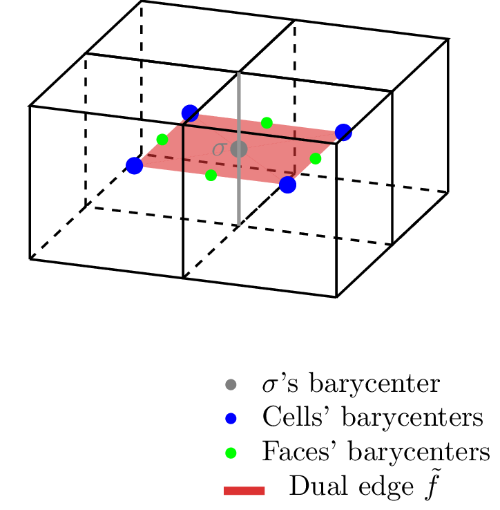
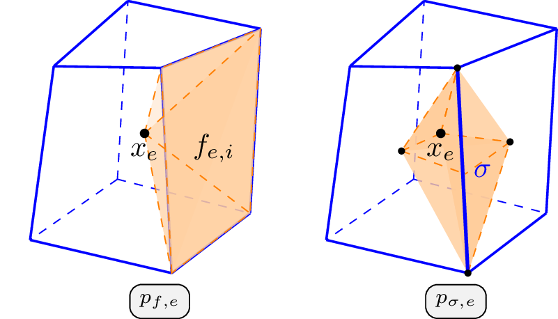
PolyMAC introduces a dual mesh. The gravity center of each control volume \(cv \in \{E, F, \Sigma, V\}\) (cells, faces, edges, vertices) is called \(x_{cv}\). The dual entities are:
| Field | Location |
|---|---|
| Pressure \(p\) | Primal cell \(e\) (= dual cell \(\widetilde{v}\)) plus an auxiliary face value \(p_f\) |
| Velocity \(u_f\) | Face-normal: \(u_f = \frac{1}{\|f\|}\int \vec{u}\cdot\vec{n}_f\,\mathrm{d}S\) |
| Vorticity \(\omega_\sigma\) | Edge-tangent in 3D: \(\omega_\sigma = \frac{1}{\|\sigma\|}\int \vec{\omega}\cdot\vec{\tau}_\sigma\,\mathrm{d}l\); vertex scalar in 2D |
Scalar fields (e.g. temperature) carry a cell DOF plus a face DOF: Champ_Elem_PolyMAC_CDO has \(n_e + n_f\) values. The face DOF is the "trace" unknown of the diffusion saddle-point (see below), exposed to Echange_contact_PolyMAC_CDO for two-problem coupling. Pressure follows the same layout.
The CDO scheme is based on exact operators that switch between localizations on the primal and dual mesh.
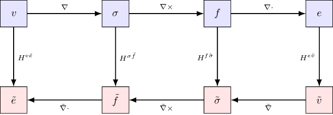
Operators are classified into two types:
Discrete gradient:
\[\text{GRAD}: V \rightarrow \Sigma, \qquad \forall \sigma \in \Sigma,\; \text{GRAD}(\mathbf{p})|_{\tilde{\sigma}} = \sum_{\tilde{v} \in V_\sigma} \iota_{v,\sigma}\,p_v \]
Discrete divergence:
\[\text{DIV}: F \rightarrow E, \qquad \forall e \in E,\; \text{DIV}(\phi)|_e = \sum_{f \in F_e} \iota_{f,e}\,\phi_f \]
Discrete curl:
\[\text{CURL}: \Sigma \rightarrow F, \qquad \forall f \in F,\; \text{CURL}(\mathbf{u})|_f = \sum_{\sigma \in \Sigma_f} \iota_{\sigma,f}\,\mathbf{u}_\sigma \]
All operators have their dual counterparts \(\widetilde{\text{GRAD}}\), \(\widetilde{\text{DIV}}\), \(\widetilde{\text{CURL}}\) on the dual mesh.
Closure between primal and dual localisations uses Hodge operators \(H_{\alpha^{-1}}^{\widetilde{\mathcal{X}}\mathcal{Y}}\), expressed using local geometry and material properties (diffusivity, viscosity). Local Hodge operators must be symmetric, locally stable and ** \(\mathbb{P}_0\)-consistent** (exact on constant fields).
Three Hodge matrices are built once at domain-discretization time and reused throughout the operators:
For cell \(e\) with \(n_f\) faces, the local reconstruction is a dense \(n_f\times n_f\) matrix combining a **consistent ( \(\mathbb{P}_0\)-exact) part** with a stabilisation correction parameterised by
\[\beta = \begin{cases} 1/D & \text{on simplices (}n_f = D + 1\text{) — DGA reconstruction} \\ 1/\sqrt{D} & \text{on general polyhedra — SUSHI reconstruction} \end{cases} \]
The choice of \(\beta\) is made per cell automatically by Domaine_PolyMAC_CDO::M2.
init_m2 dispatches between two algorithms via the global flag Option_PolyMAC_family::USE_NEW_M2:
At first call the code prints a single diagnostic line summarising the stabilisation result. The % diag / % sym / lambda fields are only populated under the OSQP path — on the default path, only the width (average stencil size per cell row) is informative.
For the elliptic equation \(-\underline{\nabla}\cdot(\underline{\underline{\kappa}}\,\underline{\nabla} T) = s\), the CDO cell-based scheme yields the saddle-point system
\[\begin{pmatrix} H_{\kappa^{-1}}^{\widetilde{F}\Sigma} & \widetilde{\mathbb{G}} \\ \mathbb{D} & 0 \end{pmatrix} \begin{bmatrix} \phi \\ p \end{bmatrix} = \begin{bmatrix} 0 \\ R_E(s) \end{bmatrix} \]
with \(\widetilde{\mathbb{G}} = -\mathbb{D}^T\). The cell unknowns \(T_e\) satisfy the discrete divergence equation; the face trace unknowns \(T_f\) satisfy a continuity equation; the two blocks are coupled through the \(W_2\) Hodge matrix (Op_Diff_PolyMAC_CDO_Elem).
The trace value \(T_f\) is exact on affine fields — this is the \(\mathbb{P}_0\)-consistency property of the local Hodge.
A non-linear variant (Op_Diff_Nonlinear_PolyMAC_CDO_Elem) adds a Le Potier / Mahamane-type monotonicity correction for high-Péclet regimes, re-evaluated at each Newton iteration through cell- and face-side residual indicators.
The viscous term in the momentum equation is not discretised directly as \(-\mu\Delta u\). Using the identity
\[-\underline{\Delta}\underline{u} \;=\; \underline{\nabla}\times\underline{\nabla}\times\underline{u} - \underline{\nabla}(\nabla\cdot\underline{u}) \;=\; \underline{\nabla}\times\underline{\omega} \quad \text{(when }\nabla\cdot u = 0\text{)} \]
and introducing the vorticity \(\underline{\omega} = \underline{\text{curl}}\,\underline{u}\) as an explicit unknown at the edges (3D) or vertices (2D), the cell-based Stokes scheme [2] reads:
Find \((\mathbf{p}^*, \phi, \mathbf{\omega}^*) \in \widetilde{V} \times F \times \Sigma\) such that
\[\begin{pmatrix} -H_{\mu^{-1}}^{\Sigma\widetilde{F}} & \widetilde{\mathbb{C}} \cdot H_{\rho^{-1}}^{F\widetilde{\Sigma}} & 0 \\ H_{\rho^{-1}}^{F\widetilde{\Sigma}} \cdot \mathbb{C} & 0 & \widetilde{\mathbb{G}} \\ 0 & -\mathbb{D} & 0 \end{pmatrix} \begin{bmatrix} \mathbf{\omega}^* \\ \phi \\ \mathbf{p}^* \end{bmatrix} = \begin{bmatrix} 0 \\ S(\rho, \underline{f}^*) \\ 0 \end{bmatrix} \]
The edge rows enforce the definition of vorticity ( \(M_1 \cdot \omega = \nu\,\text{CURL}(v)\)); the face rows enforce the viscous flux balance with \(M_2 \cdot \text{CURL}(\omega)\) on the left-hand side. The unknowns of the velocity field are \((u_f)_{f \in F} \cup (\omega_\sigma)_{\sigma \in \Sigma}\) — total \(n_f + n_\sigma\) DOFs.
The mass matrix on velocity is the \(M_2\) Hodge itself — it is not diagonal. On steady-state problems with fixed mesh, the factorisation is built once via PETSc/Cholesky and reused (Domaine_PolyMAC_CDO::init_m2solv).
The pressure gradient on faces is the simple two-point difference
\[[\vec{\nabla} p]_f \cdot \vec{n}_f \, |f| \;=\; |f|\,\varphi_f\,(p_{e_2} - p_{e_1}) \]
(Op_Grad_PolyMAC_CDO_Face), and the divergence on cells is
\[[\nabla\cdot u]_e \;=\; \sum_{f \in F_e} \sigma_{e,f}\,|f|\,\varphi_f\,u_f \]
(Op_Div_PolyMAC_CDO). The pair \((\mathbb{D}, \widetilde{\mathbb{G}} = -\mathbb{D}^\top)\) discretises the saddle-point block of the incompressible NS system. The natural primal-dual orthogonality of CDO replaces the multi-point reconstruction needed by PolyMAC_MPFA; in particular, there is no wall-pressure trace closure — walls and symmetry faces do not contribute to Op_Grad, and the right boundary closure is enforced through the \(M_2\) Hodge and the curl-curl viscous term.
The pressure-Poisson matrix used by the projection step (Assembleur_P_PolyMAC_CDO) has size \((n_e + n_f)^2\): face pressures participate as auxiliary unknowns, derived from cell pressures through the \(W_2\) Hodge during the pressure-solver step. For each cell \(e\), the local contribution is
\[M_{f f_b} \;=\; \frac{|f|\,|f_b|\,\varphi_e}{|e|}\,W_2(i, j) \]
assembled on the face-face block, with the corresponding \(-M_{e f}\) entries on the cell-face cross-blocks.
Op_Conv_Amont_PolyMAC_CDO_Elem and Op_Conv_Centre_PolyMAC_CDO_Elem are the classical first-order upwind and centred schemes on face-normal velocities:
\[\text{flux}_f = \begin{cases} \Delta t \cdot u_f \cdot |f|\,\varphi_f \cdot T_{e_{\text{up}}} & \text{(upwind)} \\ \Delta t \cdot u_f \cdot |f|\,\varphi_f \cdot \frac{T_{e_1} + T_{e_2}}{2} & \text{(centred)} \end{cases} \]
The auxiliary face trace \(T_f\) introduced by the diffusion operator is not used in convection — only cell values.
Op_Conv_EF_Stab_PolyMAC_CDO_Face is a face-based blended EF-Stab scheme:
\[\text{dfac}(j) \;=\; \frac{|f|\,u_f\,\varphi_e}{2}\,\bigl(1 + \alpha\,\mathrm{sgn}(u_f)\bigr),\qquad \alpha \in [0, 1] \]
with \(\alpha\) blending pure upwind ( \(\alpha = 1\), exposed as Op_Conv_Amont_PolyMAC_CDO_Face) and pure centred ( \(\alpha = 0\), Op_Conv_Centre_PolyMAC_CDO_Face). Two coupling paths:
This operator is single-phase only (assert(N == 1) in the code).
There is no F → cell reconstruction step inside the convection operator. The Perot face-to-cell formula
\[\vec{u}_e \;=\; \frac{1}{|e|}\sum_{f \in F_e} \sigma_{e,f}\,|f|\,(\vec{x}_f - \vec{x}_e)\,u_f \]
[2] (and Perot–Basumatary, J. Comput. Phys. 2014) is implemented in Domaine_PolyMAC_CDO::init_ve, but it is used only for output / post-processing, pressure-loss source terms, and the boundary CURL handling in the viscous operator — not inside the convective stencil.
For scalars (Champ_Elem_PolyMAC_CDO):
| BC type | Effect on the local system |
|---|---|
| Dirichlet | hard-set \(T_f = T_{\text{imp}}\); identity row on the face DOF |
| Neumann_paroi | RHS gets \(+\|f\|\,\phi_{\text{imp}}\) |
| Echange_externe_impose | RHS gets \(h\,T_{\text{ext}}\); matrix gets \(+\|f\|\,h\) on (f, f) |
| Echange_global_impose | adds friction-type term on the cell column |
| Echange_contact_PolyMAC_CDO | monolithic two-problem coupling via \(W_2\) stencil exchange — the only BC that produces matrix entries across two problems |
| Symetrie / outflow | nothing to add |
For velocity (Champ_Face_PolyMAC_CDO):
| BC type | Effect on the local system |
|---|---|
| Dirichlet ( \(\vec{u}\) imposed) | \(u_f\) hard-set in mass row; full \(\vec{u}\) vector fed to the boundary CURL via ra |
| Symetrie ( \(\vec{n}_f\cdot\vec{u} = 0\)) | \(u_f = 0\); tangential \(\omega\) handled through the va reconstruction |
| Neumann_sortie_libre (pressure imposed) | pressure Dirichlet; \(u_f\) free |
Assembling the building blocks above gives, at each Newton step, the discrete incompressible NS system
\[\begin{cases} H_{\mu^{-1}}\,\underline{\omega}^* = \underline{\nabla}\times(\rho^{-1}\underline{\phi}), \\ \partial_t(\rho^{-1}\underline{\phi}) + \nabla\cdot((\rho^{-1}\underline{\phi})\otimes(\rho^{-1}\underline{\phi})) + \rho^{-1}\underline{\nabla}\times\underline{\omega}^* + \underline{\nabla}p^* = \underline{f}^*, \\ \underline{\nabla}\cdot\underline{\phi} = 0. \end{cases} \]
The continuous-to-discrete correspondence is summarised by:
| Continuous identity | Discrete realisation |
|---|---|
| \(-\Delta u = \nabla\times\omega\) (when \(\nabla\cdot u = 0\)) | \(M_2 \cdot \text{CURL}(\omega) = \nu \cdot M_1^{-1} \cdot \text{CURL}(u)\) |
| \(\omega = \nabla\times u\) | \(M_1\,\omega = \nu\,\text{CURL}(u)\) (edge row) |
| \(\nabla\cdot u = 0\) | \(D\,u_f = 0\) (cell row) |
| \(\nabla p\) | \(-D^\top p_e\) (face row contribution) |
| \(\partial_t u\) | \(M_2 / \Delta t \cdot u_f\) (mass relation) |
This is the discrete Hodge–Helmholtz decomposition built into the geometry of the dual mesh: the CDO scheme preserves it exactly, with \(D \cdot \widetilde{G} = D \cdot (-D^\top) \equiv\) discrete pressure Laplacian.
PolyMAC_HFV is based on a Hybrid Finite Volume approach [11] [6]. It is mathematically close to PolyMAC_CDO since HFV and CDO methods are equivalent [6], but implementation-wise PolyMAC_HFV shares the architecture of PolyMAC_MPFA (only the face-flux reconstruction differs).