|
TRUST 1.9.8
HPC thermohydraulic platform
|
|
TRUST 1.9.8
HPC thermohydraulic platform
|
This page describes the architectural foundations of TRUST's parallelism: the programming model, the distributed mesh data structures, the distributed-array machinery, and the partitioning toolkit. It complements the user-facing Parallel Simulations guide — which covers how to run a parallel calculation — by explaining how the kernel is wired internally, for anyone touching the C++ sources.
TRUST runs in SPMD mode (Single Program, Multiple Data): every processor executes the same code path, and at any instant they sit at the same point in the code. All processors therefore solve the same system of equations simultaneously (same equations, same discretization, same time scheme). Whenever processors need to exchange data, they do so at synchronisation points — collective operations baked into the code.
SPMD contrasts with MPMD (Multiple Program, Multiple Data), where each processor runs a different code and inter-processor communications go through rendez-vous points — less frequent but harder to organise. For example, a hypothetical MPMD TRUST could have one processor solve Navier–Stokes while another solves a thermal problem.
In practice, TRUST is not strictly SPMD: the data each processor operates on is not always the same size (one processor's sub-domain has a different number of elements than another's), and some non-linear models (turbulence, convection operators, ...) have conditional branches whose outcome depends on local values and can therefore differ across processors.
TRUST resolves this with fine-grained MPMD blocks — short sections (loops over geometric items whose count varies per processor, loops over matrix entries, ...) that cannot contain inter-processor communications. These blocks are themselves organised in an SPMD pattern: every processor enters the same MPMD block at the same point in the code.
The TRUST kernel's high-level algorithms (operators, matrix solvers, framework methods) are coded SPMD by default. When you write such code:
TRUST theoretically supports a higher-level MPMD layer via the Process class and the notion of groups (sets of processors executing SPMD code together). A group can be the audience of an mpsum call, for instance, so the sum spans only that group's processors. The mechanism is plumbed but has only ever been used in prototype form (an AMR/dynamic-load-balancing experiment). Routinely using it would require generalising every distributed object to carry a reference to its owning group.
The computational domain is partitioned into N sub-domains: every element belongs to exactly one sub-domain. Each processor owns one sub-domain and knows about the geometric items attached to it (vertices, faces, edges, boundary faces). Those are the sub-domain's real items.
Some real items are shared with a neighbouring sub-domain — a vertex on the boundary between two sub-domains is real on both. Such shared items are called common items ("items communs"). The boundary between two sub-domains — the set of common items plus the metadata describing the link — is called a joint.
For numerical schemes computed on items adjacent to joints, a processor needs to access the values on items just across the joint, on the neighbouring sub-domain. Those extra items are virtual items ("items virtuels"). The number of layers of virtual items kept is the joint thickness ("épaisseur de joint"):
If the thickness is N, a sub-domain knows every element whose neighbours-of-neighbours-of-... (N-1 hops) include one of its real elements, plus the attached vertices/faces/edges. Two elements are "neighbours" if they share at least one common vertex.
Two conventions worth knowing when reading the code:
A distributed array ("tableau distribué") holds values indexed by geometric items. For values associated with virtual items, the array stores a copy obtained by copying the corresponding real value from the neighbour processor's sub-domain.
The conventional layout is:
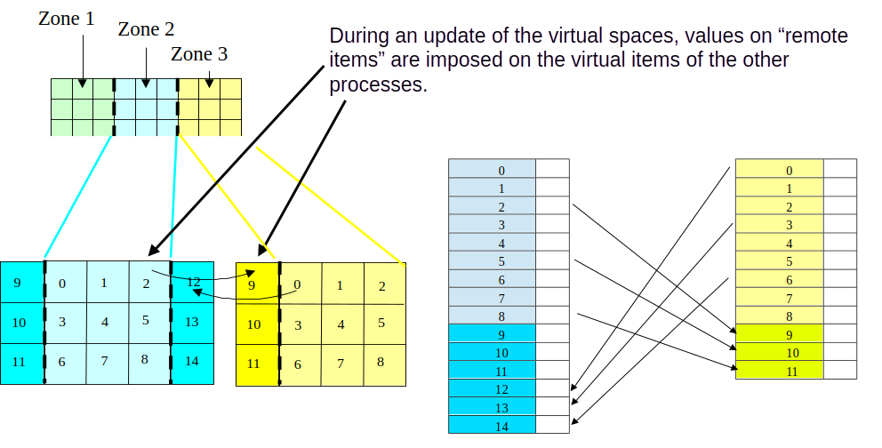
The standard pattern: every processor computes the values on its real items, then performs an "échange espace virtuel" (virtual space exchange) where it sends those real values to the neighbours that need them as virtual values, and receives the values its own virtual items expect. After this round-trip, the array's virtual section is up to date.
A few invariants:
The virtual-space layout of a distributed array is described by an MD_Vector (metadata vector) — built once per geometric type for a domain and reused by every array indexed by items of that type. The Scatter class exposes the construction sequence:
Many distributed arrays hold not numerical values but indices into other geometric arrays — e.g. for each element, the local indices of its vertices in the local-sub-domain vertex table. Naïvely running the virtual-space exchange on such an array would copy raw indices from another processor, which would point at the wrong vertices on the receiving side.
Scatter::construire_espace_virtuel_traduction(md_indice, md_valeur, tableau) handles this: it exchanges the raw indices via the md_indice layout, then translates them into the local numbering defined by md_valeur. The element-vertex table, the face-vertex table, the element-faces and face-neighbours tables all rely on this mechanism.
Each sub-domain stores its joints in a list of Joint objects, one per neighbouring sub-domain. Each Joint then carries one Joint_Items instance per geometric type, indexed by the enum class JOINT_ITEM { SOMMET, ELEMENT, FACE, ARETE, FACE_FRONT } declared in Joint.h. A Joint_Items exposes:
| Accessor | What it returns |
|---|---|
| items_distants() | Local indices of the real items this sub-domain exports as virtuals to the neighbour (ArrOfInt_t). |
| items_communs() | Local indices of the items shared (real on both sides) with the neighbour (ArrOfInt_t). |
| renum_items_communs() | Two-column index map (IntTab_t): column 0 — local index; column 1 — corresponding index on the neighbour processor. |
For initialisation, the matching set_items_distants(), set_items_communs() and set_renum_items_communs() setters return mutable references. All accessors come in templated _32_64 flavours — the _t typedefs (ArrOfInt_t, IntTab_t) resolve to the right integer width at compile time.
For each canonical mesh array, here's the convention:
The mesh cutter is organised around three classes:
Partitionneur_base::construire_partition() must produce a partition that respects periodic boundaries. Two invariants:
The renum_som_perio table must point at the same real vertex on every processor. If a vertex is multi-periodic, every processor that owns it must also own every other multi-periodic vertex associated with it. A partition that splits a multi-periodic vertex group across processors is rejected.
Similarly, a processor must not own an isolated periodic vertex: if a sub-domain contains a vertex adjacent to a periodic face, it must own at least one of the adjacent periodic faces, so the periodic vertex can be discovered by walking the faces.
To enforce these, Partitionneur_base exposes corriger_bords_avec_graphe() and corriger_bords_avec_liste(), which post-process a candidate partition until the invariants hold:
For each sub-domain it builds:
The distant items are also computed here in the current code path, but that operation is optional — it can be deferred to Scatter at load time (notably for MED-format partitions that don't ship the distant-element lists).