Quick Start

The following tutorials require a Linux-based computer.

How to install TRUST

See the instructions here.

If you need help installing TRUST, contact the TRUST support team.

Sourcing the TRUST environment

Whenever you want to use TRUST or one of its derived commands, the first thing to do is to load its environment:

source $my_path_to_TRUST_installation/env_TRUST.sh

This needs to be done in every new terminal where you want to use the TRUST binary or utilities.

How to configure TRUST

As you will see in the following, TRUST uses .data files. In order to have keywords highlighted in the .data files, we recommend the user run:

source $my_path_to_TRUST_installation/env_TRUST.sh
trust -config gedit|vim|emacs

Now you can use TRUST:

trust [option] datafile [nb_cpus] [1>datafile.out] [2>datafile.err]

You can get the list of trust command options with:

trust -help

What is a datafile

To run a TRUST simulation, all you have to do is write a correctly formatted data file. This is one of the advantages offered by the platform, allowing the user to change, modify, and test calculations without needing to write C++ code or recompile and link with the TRUST library. However, there is a specific syntax that must be respected to ensure that the TRUST interpreter can read the data file correctly and perform the necessary calculations.

We recommend using SI units for all quantities (velocity, viscosity, etc.)

Warning

TRUST is sensitive to whitespace. To avoid issues, use a space before and after each keyword. For example, Read_MED{domain dom file Mesh.med} will not work! You should write Read_MED { domain dom file Mesh.med } (note the spaces before and after the braces { ... }).

Note

It is possible to write comments in your data file using the # character, with # at the beginning and at the end of the commented line or paragraph. C++ style block comments are also supported, between /* and */. Pay attention to whitespace. Examples:

# THIS IS A COMMENT #
/* THIS ALSO */
 
/* THESE
   ARE
   ALSO
   COMMENTS */
 
# THESE
  TOO
  ...
  YES ! #
 
#THIS IS NOT GOOD! NEED SPACES#
/*THIS IS BAD TOO*/
 
// THIS IS NOT POSSIBLE
 
# THIS IS NOT POSSIBLE BECAUSE IT IS NOT CLOSED
 
/* NEITHER IS THIS

Flow around an obstacle

This first case aims to give you the basics for launching a numerical simulation with TRUST. The test case is therefore quite simple, so you can get started with TRUST smoothly.

Problem description

This first tutorial simulates the flow around a square cylinder in 2 dimensions as shown below.

The geometry used is shown in the figure below:

Geometry of the Obstacle case

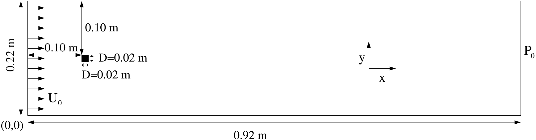
The physical properties of the fluid and boundary conditions are:

Fluid Properties	Value
Dynamic viscosity (μ)	3.7 × 10⁻⁵ kg·m⁻¹·s⁻¹
Density (ρ)	2 kg·m⁻³

Boundary Conditions	Value
Inlet velocity (U₀)	1 m·s⁻¹
Outlet pressure (P₀)	0 Pa
Square cylinder	No-slip wall
Upper and lower walls	Symmetry boundary condition

This leads to a Reynolds number: Re = U₀ × H_inlet × ρ / μ = (1 × 0.22 × 2) / (3.7 × 10⁻⁵) = 11891

Get your test case

As mentioned previously, the first thing to do is to load the environment:

source $my_path_to_TRUST_installation/env_TRUST.sh

In TRUST, we have several pre-existing non-regression test cases. You can copy a single test case by specifying its name:

trust -copy case_name

For this tutorial, we will work with the Obstacle test case. Copy it from the database using:

source $my_path_to_TRUST_installation/env_TRUST.sh
mkdir -p TRUST_tutorials
cd TRUST_tutorials
trust -copy Obstacle
cd Obstacle

The handful of trust flags used in this tutorial:

Option	Details
-copy CASE	Copy a test-case data file from the TRUST database to the current dir.
-evol	Monitor the calculation in a GUI.
-clean	Remove every file TRUST generated in the current directory.
-index	Open the TRUST resource index.
-help, -h	List every option (the live source of truth).

For the full grouped flag reference (project scaffolding, debugging, profiling, cluster submission, ...), see the TRUST command-line reference section of the introduction.

To display the options of TRUST's executable itself, run:

trust Obstacle -help_trust

You can now launch the simulation using:

trust Obstacle.data

Changing the time step value and post-processing format

Let us now explore the data file that drives the simulations. For more details regarding .data files, see the How to use a data file page.

First, edit the data file Obstacle.data:

gedit Obstacle.data &

In this simulation, we use a forward Euler scheme (explicit) for time discretization with a fixed time step of 0.005s (dt_min=dt_max). Set the time step to 0.004s.

Then, replace the keyword format lml with format lata inside the post-processing block in order to use the post-processing tool VisIt during and/or at the end of the calculation.

Visualization during the calculation

You can monitor your numerical simulation with:

trust -evol Obstacle &

This tool allows you to launch sequential calculations and visualize results.

To launch the calculation, click on the button Start computation!.

You can now visualize some values, depending on your .data file:

• Select PRESSION(X=0.13,Y=0.105) in the left list and click on Plot to draw the evolution of the pressure at the probe location.
• Check the velocity profile behind the square cylinder by plotting VITESSE_X(X=0.14,Y=0.115) and VITESSE_Y(X=0.14,Y=0.115).
• You can also visualize the residuals on the same plot: select Ri = max|dV/dt| and residu = max|Ri| using the button Plot on same, or select both graphs with the Ctrl button then click Plot.

Close the GUI.

The post-processing tool VisIt

Clean your results by running:

trust -clean

Then, relaunch your computation. Once the calculation is finished, visualize the results with VisIt:

visit &

Or by using the trust -evol tool and clicking on Visualisation in the right menu.

Now, let's configure VisIt. First, in the menu File → Open file, select Off instead of Smart for the File grouping option. For the Filter, specify *.lata to list only the lata files (results). Then save your choices in the menu Options → Save Settings.

You can now open the file Obstacle.lata with: File → Open file.

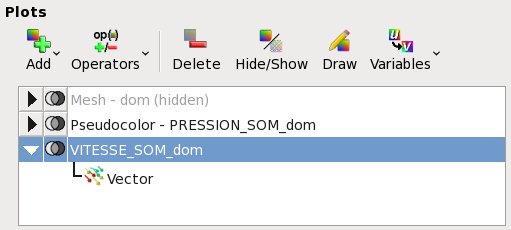
Start by visualizing the mesh in the Plots area with Add → Mesh → dom, then click on the button Draw. Zoom and move the mesh in the right window. You can zoom out with the right button (View → Reset view) or with a combination of Ctrl and the left button.

Now we can visualize the pressure field (Plots area: Add → Pseudocolor → PRESSION_SOM_dom + Draw, then select the last time on the Time slider).

You can remove or hide the mesh (select Mesh then click on Delete or Hide/Show).

Then, visualize the velocity field: Add → Vector → VITESSE_SOM_dom + Draw.

You can change each plot's attributes:

• First, click once on the small arrow ▶
• Double-click on the item Vector (see screenshot below).
• Change the number of vectors being plotted (by default 400, set it to 40000) then click on the button Make default.
• Save this modification permanently with the menu Options → Save Settings.
• Click on Apply to update, then on Dismiss to close the window.

VisIt screenshots

To save your visualization as an image, go to File → Save window. A PNG file will be created in your working directory.

Now, add a second screen with Windows → Layouts → 1x2.

In this screen, plot a horizontal pressure profile:

• Select the pressure field you want to plot.
• Right-click on the visualization and select Mode → Line out.
• Define your profile with the left button.
• Click on the origin point, hold the left button, and release at the end point.
• The profile should appear in the second window.

Note that it is necessary to update (button Draw) the right window after adding a new plot or changing an option. Automatic updates can be enabled by activating Auto apply at the top right of VisIt's GUI.

You can now create new fields (expressions) with Controls → Expressions.

VisIt also allows you to animate your visualization and/or create a movie: File → Save movie.

Another useful tool in VisIt is queries, which enable you to perform operations on your variables: Controls → Query.

Finally, save your work with: File → Save session.

To reopen it in a future VisIt session, use: File → Restore session.

During a 3D visualization, you may want to visualize a slice of your numerical simulation. To do so, use one of the available operators in Plots → Operators → Slicing → Slice.

For more information on VisIt, refer to:

• The VisIt website and its manuals
• How to contact VisIt support

Outputs and calculation resumption

Start by editing the different output (*.out) files to read the complete balances (mass, stress, energy, ...) on the whole domain or at the boundaries, for example:

• Obstacle_pb_Debit.out for mass conservation (flow rates)
• Obstacle_pb_Contrainte_visqueuse.out for viscous constraints
• Obstacle_pb_Force_pression.out for pressure forces
• Obstacle_pb_Convection_qdm.out for momentum flow rate

Then, we want to modify the data file in order to resume the calculation from where it stopped:

• First, the file Obstacle_pb.sauv must have been created during the first run.
• Open it using the evol tool:

  trust -evol Obstacle &

• Find the last backup time of the previous calculation in the .err file, or in the bottom right panel of the evol tool.

• Edit your data file with Edit data, then modify the tinit and tmax values in the time discretization scheme mon_schema.

  You should set the tinit value equal to the last time at which a backup was performed, and tmax to a greater value such as 10s.

• Then, add at the end of the problem description block (just before the last }):

  reprise binaire Obstacle_pb.sauv
  

• Save and close the window.
• Resume the calculation again with the Start computation! button. You can see that values are appended to the probes from the previous calculation.

Remark: to resume your calculation, you can also use the keyword resume_last_time instead of reprise and only change the tmax value.

Probes and fields

In this part, we will see how to add and modify probes and post-processed fields.

Start by editing the data file Obstacle.data:

gedit Obstacle.data &

Then add the following elements to the post-processing block of Obstacle.data:

• A pressure probe segment (22 probes between points (0.01, 0.12) and (0.91, 0.12)). The syntax can be similar to the line below, where the probe named sonde_pression_segment captures the pressure field (pression) every 0.005 physical seconds and contains 22 probes (points) between (0.01, 0.12) and (0.91, 0.12):

  sonde_pression_segment pression periode 0.005 segment 22 0.01 0.12 0.91 0.12
  

• A velocity probe segment (22 probes between points (0.92, 0.00) and (0.92, 0.22)) to plot the velocity profile behind the square cylinder.
• Change the field post-processing period from 1s to 0.5s (keyword dt_post).
• Add vorticity to the list of post-processed fields. To find the appropriate keyword, refer to the Keywords Reference Manual page.
• You can also access useful resources locally in the TRUST index:

  trust -index &