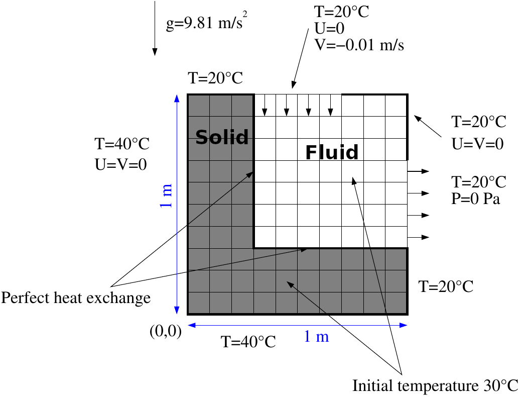
This tutorial will help you explore heat transfer between a liquid and a solid medium.

Geometry of the heat transfer case

The case we will work with in this tutorial is called docond in the TRUST non-regression database. Start by copying it into your folder:

source $my_path_to_TRUST_installation/env_TRUST.sh
mkdir -p TRUST_tutorials
cd TRUST_tutorials
trust -copy docond
mv docond Coupling_VDF
cd Coupling_VDF

Then edit the .data file and check the fluid and solid characteristics.

This coupled problem consists of 2 calculation domains. Both domains span a mesh of 10x10 cells, with \(\Delta x = \Delta y = 0.1m\).

Now open your data file with the evol tool:

trust -evol docond &

Click on Edit data and modify the data file to set the 2 domains on a mesh of 40x40 cells ( \(\Delta x= \Delta y=0.025m\)).

Note: In the block Cavite1, \(L_x=0.3\) and \(L_y=1\) and the number of nodes is 4 along X and 11 along Y.

This corresponds to a number of cells of 3 along X and 10 along Y.

Change the number of nodes for each block as follows:

First block (Cavite1): 4 11 → 13 41
Second block (Cavite2): 8 4 → 29 13
Third block (Cavite3): 8 8 → 29 29

Also replace format lml with format lata in the two problem definitions.

Click on Save and close the window. You could have achieved the same result by directly editing the docond.data file.

Run the calculation with Start computation! and check the evolution.

Then post-process the temperature field with the VisIt tool: Visualization button. A natural convection cell will appear.

Change the color tables for the temperature to use the same one on both domains. Close VisIt.

We are going to change the discretization of the test case from VDF to VEF. However, the VEF discretization only works on tetrahedra, so you first need to triangulate the domains using the keyword Trianguler_H in your .data file.

Then, give an unstructured aspect to the 2 meshes using the following syntax in your .data file:

Transformer name_of_domain x*(1-0.5*y*y) y*(1+0.1*x*y)

Substitute the keyword VDF with VEFPreP1B.

Close the evol tool and run the calculation with:

trust docond

Now, open the evol tool again:

trust -evol docond

Select \(Ri=\max_{pb1}(|dT/dt|)\), \(Ri=\max_{pb2} (|dT/dt|)\), \(Ri=\max_{pb2}(|dV/dt|)\), \(residu=max|Ri|\) with the Ctrl button and click on Plot on same.

To see when convergence is reached, select a probe, for example temperature, and click on Plot.

If the calculation takes too long, open the docond.stop file, replace the 0 with a 1 and save. The calculation will stop after the current time step and post-process the results.

Post-process the results and compare the CPU performance with the VDF discretization by checking docond.TU. Computation in VEF is approximately 10 times slower in this case.

Check the docond.out file to see the time steps for each equation: click on Edit .out at the upper right corner of the GUI.

To accelerate the calculation, make the diffusive term of each equation implicit using the diffusion_implicite keyword.

Run the calculation again without any option:

trust docond

Finally, use a fully implicit scheme by removing diffusion_implicite, then substituting Scheme_Euler_Explicit with Scheme_Euler_implicit and adding the implicit solver.

Refer to the GMRES documentation for the different options and define, following the advice given there, values for facsec and facsec_max.

Note: Your block should look like:

Solveur Implicite { solveur gmres { diag seuil 1e-30 nb_it_max 5 impr } seuil_convergence_implicite 0.01 }

Run the calculation again:

trust -evol docond