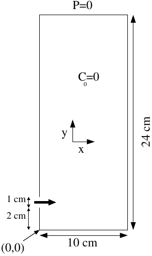
This tutorial aims at running a simulation of the tank filling test case. The test case deals with a 2D flow with Navier-Stokes and the equation for one constituent.

Geometry of the 2D tank case

The following table summarizes the parameters of the simulation:

Fluid Properties	Value
Dynamic viscosity ( \(\mu\))	\( 10^{-3}\) \(kg \cdot m^{-1} \cdot s^{-1}\)
Density ( \(\rho\))	\(1000\) \(kg \cdot m^{-3}\)
Diffusion ( \(D\))	\(10^{-9}\) \(m^{2}\cdot s^{-1}\)

Boundary Conditions	Value
Inlet velocity ( \(V(t)\))	\(\begin{cases} 1 -(y-0.025/0.005)^{2} & ,\; t \leq 0.5s \\ 0 & ,\; t>0.5s \end{cases}\)
Concentration ( \(C\))	\( \begin{cases} 1 & ,\; t \leq 0.5s \\ 0 & ,\; t>0.5s \end{cases}\)
Outlet pressure ( \(P_0\))	\(0\) \(Pa\)
Wall velocity	V= 0

Initial conditions	Value
Velocity ( \(V(x,y,t=0)\))	\(0 m \cdot s^{-1}\)
Concentration ( \(C(x,y,t=0)\))	0

You can copy the study named diagonale:

source $my_path_to_TRUST_installation/env_TRUST.sh
mkdir -p TRUST_tutorials
cd TRUST_tutorials
trust -copy diagonale

Now, edit the diagonale.data file.

Then, modify the fluid characteristics to the one given in the above table ( \(\mu, \rho, D\)).

You then need to modify the geometry parameters, so that your geometry resembles the figure below.

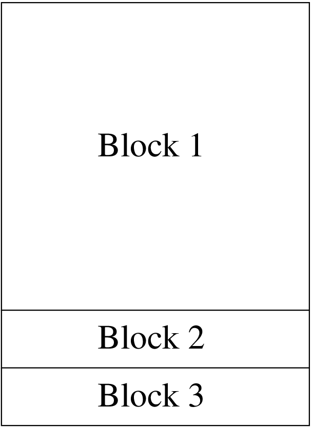
Mesh blocks of the 2D tank filling case

To do so, you have to create three blocks, starting with \(dx=dy=0.2cm\) which gives a total nodes number \(Nx=51\) and \(Ny=121\).

The first block,Block1, whose origin is (0, 0.03), \(Nx=51\), \(Ny=106\) (for \(dx=dy=0.2cm\)), \(L=0.1 m\), \(H=0.21 m\). Name the wall boundaries Left1, Outlet(=Top1) and Right1. (Don't forget the comma between block definitions.)
The second block, Block2, whose origin is (0, 0.02), \(Nx=51\), \(Ny=6\) (for \(dx=dy=0.2cm\)), \(L=0.1 m\), \(H=0.01 m\). Name the wall boundaries Inlet(=Left2) and Right2.
The third block, Block3, whose origin is (0, 0), \(Nx=51\), \(Ny=11\) (for \(dx=dy=0.2cm\)), \(L=0.1 m\), \(H=0.02 m\). Name the wall boundaries Left3, Bottom3 and Right3.

Then, define the boundary wall, using the keyword regroupebord.

You could also use facteurs, symx and symy keywords to define a refined mesh near the walls.

Once you are done with the geometry, change the values in the time scheme to stop the calculation at 1 second, and modify dt_min and dt_max values to let TRUST compute at least one time step.

Now, set the gravity value to \(-9.81 m.s^{-2}\) along the y-axis.

Note that the beta_co keyword may be useful in order to have a Boussinesq coupling between momentum and concentration equations ( \(\beta C_0 g(C-C_0\)) source term added to the Navier-Stokes equations).

Boundary and initial conditions

You need to change the initial and boundary conditions for Navier-Stokes equations:

for the Outlet boundary, impose \(P=0\),
for the Wall boundary, impose \(V_x=V_y=0\) with paroi_fixe keyword,
for the Inlet boundary, impose \((V_{x},V_{y})=(V(t),0)\) with:

\(V(t)= \begin{cases} 1-(y-0.025/0.005)^{2} & ,\; t\leq0.5s\\ 0 & ,\; t>0.5s \end{cases}\).

You will use the champ_front_fonc_txyz keyword for the velocity, to write something like: **Champ_Front_Fonc_txyz \(2\) \((1-((y-0.025)/0.005)^2)*(t<0.5)\) \(0.\)**
Note
Use ( \(t[0.5\)) syntax if you prefer ( \(t<=0.5\))

For Convection_diffusion_Concentration, you need to use:
For the Outlet, use the following keywords to ensure the external concentration is 0:

Frontiere_ouverte C_ext Champ_front_uniforme 1 0.
For the Wall, the keyword for impermeable boundary condition for concentration is paroi.
for the Inlet boundary condition of concentration, champ_front_fonc_txyz field

Then make sure to check that you have high-order schemes (i.e. Quick scheme) used in both equations to reduce numerical diffusion.

You can also neglect the diffusion term in concentration equation rather than using a small diffusion coefficient with:

Diffusion { negligeable }

Post-processing tools

To see the time evolution of velocity and concentration:

Add a concentration probe near the inlet (e.g. at (0,0.025)) (period 0.01s).
Add a velocity segment of probes (with 5 points between (0,0.021) and (0,0.029)) at the inlet boundary (period 0.01s).

Now, you are ready to run the study and follow the time evolution with the probes:

trust -evol diagonale

Press the Start computation! button and Plot or Plot on same for probes.

You can now check the flow rate at the inlet boundary in the diagonale\_pb\_Debit.out file (plotted on the right of the evol window). You should find a value close to \(6.8 \; 10^{-3} m^2.s^{-1}\).

Use VisIt to post-process the results at \(t=0.2s\), \(t=0.4s\) and \(t=0.7s\). VisIt has some useful features for this study. It can, for example, display a concentration histogram to assess the numerical diffusion in the concentration equation.

To do so, click on Add → Histogram → CONCENTRATION\_ELEM\_dom.

The volume of colored water (in \(m^3\)) is given by \(Vol(t)= 6.66.10^{-3} t\) before \(t=0.5s\) and \(Vol(t)=3.33.10^{-3}\) after.

VEF calculation

You will now create a variant of your test case.

First, copy diagonale.data to diagonale_VEF.data.

In this new file, change the discretization from VDF to VEFPreP1B. Since the VEF discretization only works on simplices, you need to triangulate your mesh by adding the trianguler keyword in your diagonale_VEF.data.

Change the keyword quick (which is only available in VDF) to muscl in order to use a MUSCL scheme.

You can also switch GCP solver to Cholesky solver of the Petsc library: GCP { precond ssor { omega 1.5 } seuil 1.e-6 } → Petsc Cholesky { }. The Cholesky method is a direct method that works well on relatively small cases but that may need a large amount of RAM memory for larger problems.

Run the calculation.

You should encounter an error, and TRUST will stop the calculation. You will find a diagonale_VEF.decoupage_som file in your working directory.

As TRUST indicates, to avoid this problem, you can:

change the trianguler keyword to trianguler_h,
or use the verifiercoin keyword.

The first method is straightforward and works here due to the geometry of your domain.

To use the second one, you will need the diagonale_VEF.decoupage_som file. Add the following: VerifierCoin dom { read_file diagonale_VEF.decoupage_som } in your diagonale\_VEF.data, just after trianguler dom. This will subdivide any inconsistent 2D/3D cells.

Finally, run both of your .data files and compare the results between VDF/quick and VEFPreP1B/muscl.