Quick start#
The following tutorials require a Linux-based computer.
How to install TRUST#
See the instructions here.
If you need help installing TRUST, contact the TRUST support team.
Sourcing the TRUST environment#
Whenever you want to use TRUST or one of its derived commands, the first thing to do is to load its environment:
source $my_path_to_TRUST_installation/env_TRUST.sh
This needs to be done in every new terminal where you want to use the TRUST binary or utilities.
How to configure TRUST#
As you will see in the following, TRUST uses .data files. In order to have keywords highlighted in the .data files, we recommend the user run:
source $my_path_to_TRUST_installation/env_TRUST.sh
trust -config gedit|vim|emacs
Now you can use TRUST:
trust [option] datafile [nb_cpus] [1>datafile.out] [2>datafile.err]
You can get the list of trust command options with:
trust -help
What is a datafile#
To run a TRUST simulation, all you have to do is write a correctly formatted data file. This is one of the advantages offered by the platform, allowing the user to change, modify, and test calculations without needing to write C++ code or recompile and link with the TRUST library. However, there is a specific syntax that must be respected to ensure that the TRUST interpreter can read the data file correctly and perform the necessary calculations.
We recommend using SI units for all quantities (velocity, viscosity, etc.)
Warning
TRUST is sensitive to whitespace. To avoid issues, use a space before and after each keyword. For example, Read_MED{domain dom file Mesh.med} will not work! You should write Read_MED { domain dom file Mesh.med } (note the spaces before and after the braces { … }).
Note
It is possible to write comments in your data file. This can be done using the # character, with # at the beginning and at the end of the commented line or paragraph. It is also possible to enclose comments between /* and */, as with block comments in C++. Again, pay attention to whitespace. See these examples:
# THIS IS A COMMENT #
/* THIS ALSO */

/* THESE
	ARE
	ALSO
	COMMENTS */

# THESE
	TOO
	...
	YES ! #

#THIS IS NOT GOOD! NEED SPACES#
/*THIS IS BAD TOO*/

// THIS IS NOT POSSIBLE

# THIS IS NOT POSSIBLE BECAUSE IT IS NOT CLOSED

/* NEITHER IS THIS
Flow around an obstacle#
This first case aims to give you the basics for launching a numerical simulation with TRUST. The test case is therefore quite simple, so you can get started with TRUST smoothly.
Problem description#
This first tutorial simulates the flow around a square cylinder in 2 dimensions as shown below.

The geometry we use is shown in Figure 1
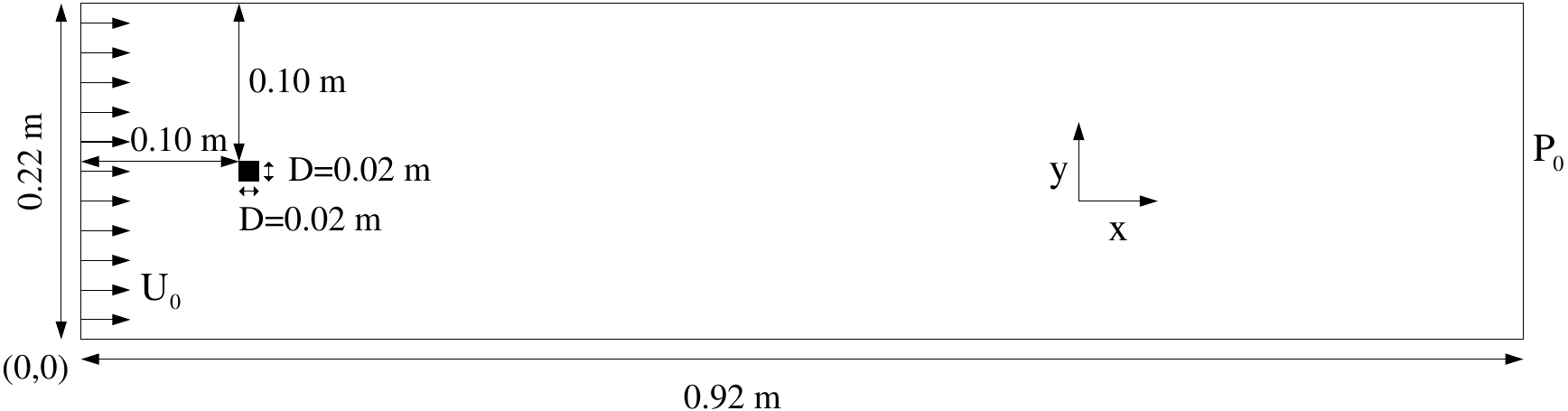
Figure 1 Geometry of the Obstacle case#
The physical properties of the fluid and boundary conditions are:
Fluid Properties |
Value |
|---|---|
Dynamic viscosity (\(\mu\)) |
\(3.7 \times 10^{-5}\) \(kg \cdot m^{-1} \cdot s^{-1}\) |
Density (\(\rho\)) |
\(2\) \(kg \cdot m^{-3}\) |
Boundary Conditions |
Value |
|---|---|
Inlet velocity (\(U_0\)) |
\(1\) \(m \cdot s^{-1}\) |
Outlet pressure (\(P_0\)) |
\(0\) \(Pa\) |
Square cylinder |
No-slip wall |
Upper and lower walls |
Symmetry boundary condition |
This leads to a Reynolds number for this simulation: \(Re = \frac{U_0 H_{inlet} \rho}{\mu} = \frac{1\times 0.22 \times 2}{3.7 \; 10^{-5}} = 11891\)
Get your test case#
As mentioned previously, the first thing to do is to load the environment:
source $my_path_to_TRUST_installation/env_TRUST.sh
In TRUST, we have several pre-existing non-regression test cases. You can copy a single test case by specifying its name:
trust -copy case_name
For this tutorial, we will work with the Obstacle test case. Therefore, copy the test case from the database using:
source $my_path_to_TRUST_installation/env_TRUST.sh
mkdir -p TRUST_tutorials
cd TRUST_tutorials
trust -copy Obstacle
cd Obstacle
To get the full help for the trust command, run:
trust -help
Here is a panel of some available options:
Option |
details |
|---|---|
-help|-h |
Displays available options. |
-baltik [baltik_name] |
Instantiates an empty Baltik project. |
-index |
Access to the TRUST resource index. |
-config vim|emacs|gedit |
Configure vim, emacs or gedit to recognize TRUST keyword syntax. |
-trustify |
Check the data file’s keywords with trustify. |
-eclipse-trust |
Generate Eclipse configuration files to import TRUST sources. |
-eclipse-baltik |
Generate Eclipse configuration files to import BALTIK sources. |
-evol |
Monitor the TRUST calculation (GUI). |
-jupyter |
Create a basic Jupyter notebook. |
-clean |
Clean the current directory of all files generated by TRUST. |
-search keywords |
List the test cases in the database which contain the given keywords. |
-copy |
Copy the test case data file from the TRUST database to the current directory. |
-check all|testcase|list |
Check the non-regression of all test cases, a single test case, or a list of test cases specified in a file. |
-ctest all |
Similar to -check but using ctest. |
-gdb |
Run under the gdb debugger. |
-valgrind |
Run under valgrind. |
-heaptrack |
Run heaptrack (heap profiler). |
-advisor |
Run the advisor tool (vectorization). |
-vtune |
Run the vtune tool (profiling). |
-perf |
Run the perf tool (profiling). |
-trace |
Run the traceanalyzer tool (MPI profiling). |
-create_sub_file |
Create a submission file only. |
datafile -help_trust |
Print options of TRUST_EXECUTABLE [CASE[.data]] [options]. |
To display the options of TRUST’s executable, run:
trust Obstacle -help_trust
You can now launch the simulation using:
trust Obstacle.data
Changing the time step value and post-processing format#
Let us now explore the data file that drives the simulations. For more details regarding .data files, go to How to use a data file.
First, edit the data file Obstacle.data:
gedit Obstacle.data &
In this simulation, we use a forward Euler scheme (explicit) for time discretization with a fixed time step of 0.005s (dt_min=dt_max). Set the time step to 0.004s.
Then, replace the keyword format lml with format lata inside the post-processing block in order to use the post-processing tool VisIt during and/or at the end of the calculation.
Visualization during the calculation#
You can monitor your numerical simulation with:
trust -evol Obstacle &
This tool allows you to launch sequential calculations and visualize results.
To launch the calculation, click on the button Start computation!.
You can now visualize some values, depending on your .data file:
Select
PRESSION(X=0.13,Y=0.105)in the left list and click onPlotto draw the evolution of the pressure at the probe location.Check the velocity profile behind the square cylinder by plotting
VITESSE_X(X=0.14,Y=0.115)andVITESSE_Y(X=0.14,Y=0.115).You can also visualize the residuals on the same plot: select \(Ri = max \left| \frac{dV}{dt} \right|\) and \(residu = max \left| Ri \right|\) using the button
Plot on same, or select both graphs with theCtrlbutton then clickPlot.
Close the GUI.
The post-processing tool VisIt#
Clean your results by running:
trust -clean
Then, relaunch your computation. Once the calculation is finished, visualize the results with VisIt:
visit &
Or by using the trust -evol tool and clicking on Visualisation in the right menu.
Now, let’s configure VisIt. First, in the menu File \(\rightarrow\) Open file, select Off instead of Smart for the File grouping option. For the Filter, specify *.lata to list only the lata files (results). Then save your choices in the menu Options \(\rightarrow\) Save Settings.
You can now open the file Obstacle.lata with: File \(\rightarrow\) Open file.
Start by visualizing the mesh in the Plots area with Add \(\rightarrow\) Mesh \(\rightarrow\) dom, then click on the button Draw. Zoom and move the mesh in the right window. You can zoom out with the right button (View \(\rightarrow\) Reset view) or with a combination of Ctrl and the left button.
Now we can visualize the pressure field (Plots area: Add \(\rightarrow\) Pseudocolor \(\rightarrow\) PRESSION_SOM_dom + Draw, then select the last time on the Time slider).
You can remove or hide the mesh (select Mesh then click on Delete or Hide/Show).
Then, visualize the velocity field:
Add \(\rightarrow\) Vector \(\rightarrow\) VITESSE_SOM_dom + Draw.
You can change each plot’s attributes:
First, click once on the small arrow \(\blacktriangleright\)
Double-click on the item Vector (see Figure 2).
Change the number of vectors being plotted (by default 400, set it to 40000) then click on the button
Make default.Save this modification permanently with the menu
Options\(\rightarrow\)Save Settings.Click on
Applyto update, then onDismissto close the window.
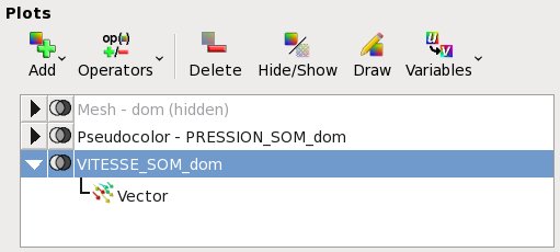
Figure 2 VisIt screenshots#
To save your visualization as an image, go to File \(\rightarrow\) Save window. A PNG file will be created in your working directory.
Now, add a second screen with Windows \(\rightarrow\) Layouts \(\rightarrow\) 1x2.
In this screen, plot a horizontal pressure profile:
Select the pressure field you want to plot.
Right-click on the visualization and select
Mode\(\rightarrow\)Line out.Define your profile with the left button.
Click on the origin point, hold the left button, and release at the end point.
The profile should appear in the second window.
Note that it is necessary to update (button Draw) the right window after adding a new plot or changing an option. Automatic updates can be enabled by activating Auto apply at the top right of VisIt’s GUI.
You can now create new fields (expressions) with Controls \(\rightarrow\) Expressions.
VisIt also allows you to animate your visualization and/or create a movie: File \(\rightarrow\) Save movie.
Another useful tool in VisIt is queries, which enable you to perform operations on your variables: Controls \(\rightarrow\) Query.
Finally, save your work with: File \(\rightarrow\) Save session.
To reopen it in a future VisIt session, use: File \(\rightarrow\) Restore session.
During a 3D visualization, you may want to visualize a slice of your numerical simulation. To do so, use one of the available operators in Plots \(\rightarrow\) Operators \(\rightarrow\) Slicing \(\rightarrow\) Slice.
For more information on VisIt, you can refer to:
How to contact VisIt support
Outputs and calculation resumption#
Start by editing the different output (*.out) files to read the complete balances (mass, stress, energy, …) on the whole domain or at the boundaries, for example:
Obstacle_pb_Debit.out for mass conservation (flow rates)
Obstacle_pb_Contrainte_visqueuse.out for viscous constraints
Obstacle_pb_Force_pression.out for pressure forces
Obstacle_pb_Convection_qdm.out for momentum flow rate
Then, we want to modify the data file in order to resume the calculation from where it stopped:
First, the file
Obstacle_pb.sauvmust have been created during the first run.Open it using the
evoltool:trust -evol Obstacle &
Find the last backup time of the previous calculation in the
.errfile, or in the bottom right panel of theevoltool.Edit your data file with
Edit data, then modify the tinit and tmax values in the time discretization schememon_schema.You should set the tinit value equal to the last time at which a backup was performed, and tmax to a greater value such as 10s.
Then, add at the end of the problem description block (just before the last
}):reprise binaire Obstacle_pb.sauv
Save and close the window.
Resume the calculation again with the
Start calculation!button. You can see that values are appended to the probes from the previous calculation.
Remark: to resume your calculation, you can also use the keyword resume_last_time instead of reprise and only change the tmax value (cf euler_scheme).
Probes and fields#
In this part, we will see how to add and modify probes and post-processed fields.
Start by editing the data file Obstacle.data:
gedit Obstacle.data &
Then add the following elements to the post-processing block of Obstacle.data:
A pressure probe segment (22 probes between points (0.01, 0.12) and (0.91, 0.12)). The syntax can be similar to the line below, where the probe named sonde_pression_segment captures the pressure field (pression) every 0.005 physical seconds and contains 22 probes (points) between (0.01, 0.12) and (0.91, 0.12):
sonde_pression_segment pression periode 0.005 segment 22 0.01 0.12 0.91 0.12
A velocity probe segment (22 probes between points (0.92, 0.00) and (0.92, 0.22)) to plot the velocity profile behind the square cylinder.
Change the field post-processing period from 1s to 0.5s (keyword dt_post).
Add vorticity to the list of post-processed fields. To find the appropriate keyword, refer to Existing & predefined fields.
You can also access useful resources locally in the TRUST index. Take a few minutes to find test cases containing a particular keyword using the Keywords link in:
trust -index &