Unlike PolyMAC, PolyMAC_MPFA (previously named PolyMAC_P0) does not introduce the vorticity. Moreover, no
complex dual mesh is explicitly needed. The location of the unknowns is
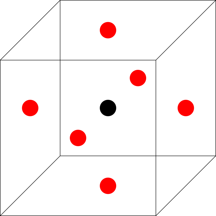
described in Figure 17.
Figure 17 Location of the unknowns when using PolyMAC_P0#
PolyMAC_P0 is based on Multi Point Flux Approximation (MPFA) method.
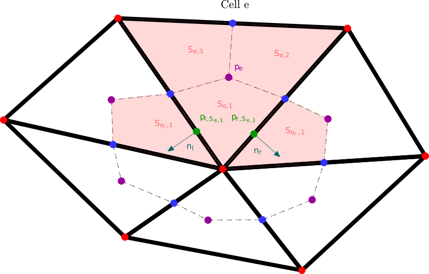
The choice of the method is based on a coercivity condition. Let’s briefly introduce the core ideas of gradient approximation using MPFA methods. First, a dual mesh is constructed. An exemple of dual mesh for a tringular mesh is presented in Figure 18, where the red dot are the primal vertices and black lines the primal faces. The procedure to build the dual mesh in Figure 18 is as follows:
Link each cell’s (\(e\)) gravity center (in purple) to the gravity center of each cell’s face \(f \subset e\) ( in blue). Doing so, the face of the mesh are cut into two sub-faces called \(\hat{f}_1\) and \(\hat{f}_2\). Each cell can then be subdivided into \(N_i\) quadrilaterals (in orange), called \((S_{e,i})_{i\in\{ 1,\dots, N_i \} }\).
Introduce for each sub-face \(\hat{f} \subset f\), an auxiliary quantity ( in green). For the MPFA-symmetric method, those auxiliary quantities are set at one third and two third of the face \(f\). For the MPFA-O method, they are put at the center of the face, however, the value of the auxiliary unknowns at the center is not continuous. The MPFA-O(\(\eta\)) method can be seen as an in between, as it try compute the optimum location of the auxiliary unknown.
Figure 18 Construction of a gradient using MPFA method#
On \(S_1\) in Figure 18 for example, the gradient of a potential p, \(G_{S_{e,i}}([p]_e)\) is computed as:
where \(\vec{n_1}\) and \(\vec{n_2}\) are the outward unit normal vectors of the respective sub-faces \(\tilde{f}\subset f\) where the auxiliary elements \(p_{S_{e,1}}\) and \(p_{S_{e,2}}\) are located. Thus, \(G^{\text{MPFA}}\) writes:
(8)#\[G^{\text{MPFA}}: [p]_e \mapsto G^{\text{MPFA}}([p]_e) \ , \quad \forall e \in E \ , \quad i \in S_e \ : \quad G^{\text{MPFA}} _{|S_{e,i}} = G_{S_{e,i}}([p]_e).\]
A core assumption of the MPFA method is to suppose that \(G^{\text{MPFA}}([p]_e)\) is constant on each \(S_{e,i}\). When enforcing the continuity across the sub-faces that are linked by a vertex of the primal mesh, auxiliary variables can be substitute by cells unknowns.
The MPFA methods are impemented in Domaine_PolyMAC_P0::fgrad.
(9)#\[\begin{split}\begin{aligned}
& \partial_{t} \left( u \right) + \nabla \cdot \left( u \otimes u \right) + \nabla p - \mu \Delta u = f \ , \\
& \nabla \cdot u = 0 \ .\end{aligned}\end{split}\]
The mass equation is discretised at the cell using the Green-Ostrogradski theorem:
\[|e|[\nabla \cdot u]_e = |f| \sum _{F_e} [u]_f\]
The momentum equation is discretised at the face:
For the convective term:
Approximate the value of the velocity at the cell:
with \(\beta \in [0,1]\) and \(\gamma \in \{0,1\}\) such that \(\gamma =1\) if \([u_f]\geq 0\) and \(0\) otherwise.
The convective terms:
Interpolate convective terms to the face:
\[[\nabla \cdot (u\otimes u)]_{f} = \lambda_{e,f} [\nabla \cdot (u \otimes u)]_{e} + \lambda_{e',f} [\nabla \cdot (u \otimes u)]_{e'}\]
with the penalty coefficient \(\lambda_{e,f} = \frac{ |\vec{x}_{e' \rightarrow f}|}{|\vec{x}_{e' \rightarrow f}| + |\vec{x}_{e \rightarrow f}|}\), with \(e'\) the neighbouring cell of \(e\) sharing the face \(f\).
The gradient of p is computed using an MPFA scheme (8).
The diffusive term is rewritten as :
\[\Delta u = \nabla \cdot ( \nabla u + \left(\nabla u)^{\intercal} \right) )\]
Then a second order interpolation is used to compute the velocity at the cell, see:
First, introducing \(n_f\) the outward normal of face \(f\), one can write the series expansion:
Then considering the stencil composed of the faces that share a vertex of \(e\), called \(\mathcal{F}^v_e\), one can obtain the following system:
\[A \cdot U_e = U_{\mathcal{F}^v_e}\]
where each line \(i\) corresponds to the equation for the \(i^{th}\) face of \(\mathcal{F}^v_e\). \(A\) is a matrix of geometrical quantities, \(U_e\) stores the components of \(u_e\) and \((\nabla u)_e\), and \(U_{\mathcal{F}^v_e}\) the value of \(u_f\) at the face.
However, there is a large number of equations relative to the number of unknowns. To solve this problem, we use a least squares method to find the solution that minimizes:
PolyMACP0P1NC is based on a Hybrid Finite Volmue (HFV) approach, such as the one presented in [Eymard et al., 2007] and [Eymard et al., 2010]. PolyMAC_P0_P1_NC is mathematically close to the first PolyMAC, as HFV and CDO method are equivalent, see [Droniou et al., 2010].