Mesh for coupled problems#
This exercise demonstrates creating meshes for coupled multi-domain problems where interface connectivity is critical.
Problem Description#
Consider the cooling of a solid block by a fluid flowing through circular cross-section channels. The channel is centered within a square cross-section block. The outer boundaries of the solid are adiabatic.
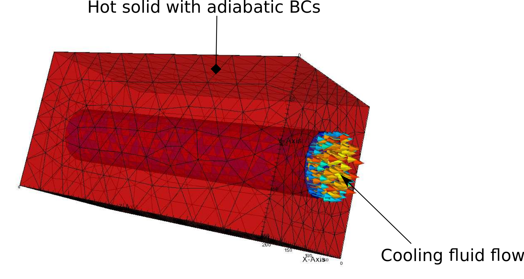
Two domains need to be created:
Domain 1: Solid block
Domain 2: Fluid channel
Key requirement: Mesh elements must be connected at the interface between domains for TRUST to read the mesh correctly.
Setup#
mkdir -p TRUST_tutorials/salome/exo4
cd TRUST_tutorials/salome/exo4
$PathToSALOME/salome &
Create a new study: File → New
Select the Geometry module
Save frequently in HDF format
Creating the Geometry#
Create the solid block: New Entity → Primitives → Box
Dx =
200, Dy =200, Dz =400Click “Apply and Close”
Create a vertex for the cylinder base: New Entity → Basic → Point
X =
100, Y =100, Z =0Click “Apply and Close”
Create the fluid channel: New Entity → Primitives → Cylinder
Base Point: Vertex_1
Vector: OZ
Radius R =
40Height H =
400Click “Apply and Close”
Cut the cylinder from the block: Operations → Boolean → Cut
Main Object: Box_1
Tool Objects: Cylinder_1
Click “Apply and Close”
Create a partition: Operations → Partition
Objects: Select both Cylinder_1 and Cut_1
Click “Apply and Close”
Note: This partition ensures mesh connectivity at the interface.
Defining Volume Groups#
Create groups for each domain:
Solid domain: New Entity → Group → Create Group
Shape Type: Volume
Name:
SolidMain Shape: Partition_1
Select the hollow box
Click “Add” → “Apply”
Fluid domain: Continue in the same dialog
Name:
FluidMain Shape: Partition_1
Select the cylindrical channel
Click “Add” → “Apply and Close”
Defining Boundary Groups#
Create surface groups for all boundaries:
Fluid inlet: New Entity → Group → Create Group
Shape Type: Surface
Name:
Fluid_inletMain Shape: Partition_1
Select the bottom of the cylinder → “Add” → “Apply”
Fluid outlet:
Name:
Fluid_outletSelect the top circular boundary → “Add” → “Apply”
Solid top:
Name:
Solid_topSelect the top of the box → “Add” → “Apply”
Solid bottom:
Name:
Solid_bottomSelect the bottom of the box → “Add” → “Apply”
Solid lateral walls:
Name:
Solid_lateral_wallsSelect the four lateral boundaries of the box → “Add” → “Apply”
Solid-Fluid interface:
Name:
Solid_Fluid_InterfaceSelect the top of the box → “Hide selected”
Select a lateral boundary → “Hide selected”
The lateral surface of the cylinder should now be visible
Select it → “Add” → “Apply and Close”
Creating the Mesh#
Switch to the Mesh module
Create the mesh: Mesh → Create Mesh
Name:
Mesh_1Geometry: Partition_1
3D algorithm: NETGEN 1D-2D-3D
Configure parameters:
Click the wheel icon next to “Hypothesis” → “NETGEN 3D Parameters”
In “Arguments”: Change fineness from “Moderate” to “Fine”
Click “OK” → “Apply and Close”
Compute the mesh:
Right-click on “Mesh_1” → Compute
Verify groups:
Check that six boundaries appear under “Group of Faces” of Mesh_1
Check that two volume groups appear under “Group of Volumes” of Mesh_1
Exporting the Mesh#
Export to MED format:
Select “Mesh_1”
Right Click → Export → MED file
Choose MED 3.2 if possible
Save as
Mesh_1.med
Dump the study: File → Dump Study
Save as a Python script (needed for the next exercise)
Running the Coupled Problem#
Copy and run the TRUST data file:
cp $TRUST_ROOT/doc/TRUST/exercices/salome/Coupled_pb.data .
trust Coupled_pb.data
Visualize the results with VisIt:
visit -o Coupled_pb.lata
Plot the temperature field on both domains and set the color bar min/max to 300 and 400 respectively. You will observe the solid cooling over time. Given sufficient simulation time, the solid temperature will eventually match the fluid temperature at steady state.