Quasi Compressible flows#
As always when using TRUST, start by loading your TRUST environment, see.
The case we will work with in this tutorial is called TP_Temp_QC_VEF in the TRUST non-regression database. It is a 2D simulation of helium gas flow in a rectangular channel from left to right between two heated walls.
Start by copying it into your folder:
source $my_path_to_TRUST_installation/env_TRUST.sh
mkdir -p TRUST_tutorials
cd TRUST_tutorials
trust -copy TP_Temp_QC_VEF
Then, open the TRUST Keyword Reference Manual in another tab, as it will be useful for looking up keywords throughout this exercise.
Edit the data file with your favorite editor, or using gedit:
gedit TP_Temp_QC_VEF.data &
You will make several changes to the .data file:
First, modify the geometry and the mesh as shown in Figure 22.
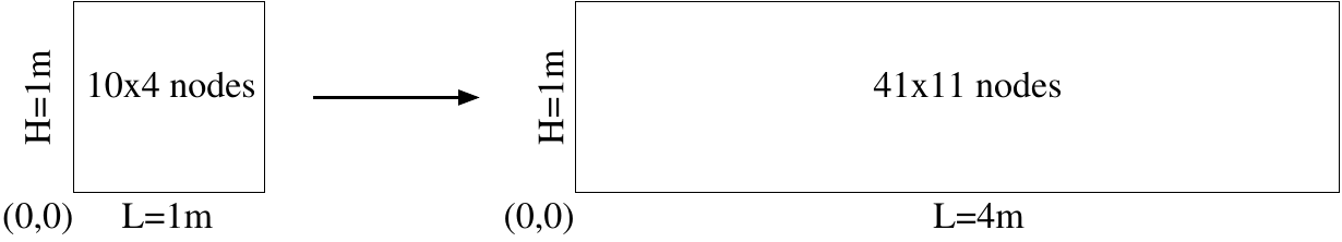
Figure 22 Geometry modification for the Low-Mach case#
Then, add several probes (velocity, density, temperature) near the upper right corner of the geometry at location (x,y)=(4,1).
Add a segment of probes (with 9 points) between locations (x,y)=(4,0.05) and (x,y)=(4,0.95) for the temperature field.
Write the results in lata format and change the dt_post period to 1s.
The goal of the calculation is to reach steady state, so remove the tmax keyword and change the seuil_statio \(\varepsilon\) value to 10 (\(|dT/dt|<\varepsilon\) and \(dt \sim 0.001s\), so \(|dT|<0.01\)).
Add the keyword impr to the pressure solver to print the convergence residuals of the solver.
Save and close your
.datafile.Run the simulation with the
evoltool (or using command lines):trust -evol TP_Temp_QC_VEF &
Check the mass flow rate (absolute and relative values) in the
TP_Temp_QC_VEF.outfile.Once the calculation is finished, visualize the results using VisIt:
visit -o TP_Temp_QC_VEF.lata &
Display the mesh and visualize the temperature field by selecting the last time step with the slider, then plot it:
Add\(\rightarrow\)Pseudo Color\(\rightarrow\)TEMPERATURE_SOM_dom\(\rightarrow\)Draw.Hide the mesh and visualize the velocity field:
Add\(\rightarrow\)Vector\(\rightarrow\)VITESSE_SOM_dom\(\rightarrow\)Draw.Save a screenshot of your visualization:
File\(\rightarrow\)Set Save options\(\rightarrow\)File type\(\rightarrow\)Select a type\(\rightarrow\)Save. An image file namedvisit***will be created in your working directory.Add a second screen with
Window\(\rightarrow\)Layout\(\rightarrow\)1x2and plot a horizontal temperature profile. To do so, select the temperature field, right-click and selectMode\(\rightarrow\)Lineout, then define your profile with the left button. The profile should appear in the second window.Close VisIt.
Going back to your .data file, replace the time scheme with an implicit time scheme such as schema_euler_implicite.
Use the implicite solver and specify the facsec and facsec_max parameters according to the advice given in facsec_expert.
Run the calculation again with this time scheme using the evol tool or with:
trust TP_Temp_QC_VEF.data 1>TP_Temp_QC_VEF.out 2>TP_Temp_QC_VEF.err
You can edit the files containing information about the time step and residual evolution for each equation:
gedit TP_Temp_QC_VEF.dt_ev &
If everything looks correct, try to improve the convergence speed of the implicit solver by adjusting the seuil_convergence_implicite keyword.
If the number of GMRES iterations is between 3 and 5, convergence is fast enough. You can find this information in the TP_Temp_QC_VEF.out file.
To resume the calculation, change the tinit value in the data file to the one saved in the .err file. You also need to insert the keyword reprise binaire TP_Temp_QC_VEF_pb.sauv in the problem definition block of your .data file.
Then, restart the calculation with:
trust TP_Temp_QC_VEF.data 1>TP_Temp_QC_VEF.out 2>TP_Temp_QC_VEF.err
or
trust -evol TP_Temp_QC_VEF.data &
The evol option automatically creates the TP_Temp_QC_VEF.out and TP_Temp_QC_VEF.err files.