Discontinuous Galerkin Methods

Discontinuous Galerkin (DG) methods form a class of finite element methods particularly suited for solving partial differential equations. Unlike standard continuous Galerkin methods, DG allows for discontinuities between elements, providing greater flexibility and robustness, especially for complex geometries or highly dynamic phenomena.

DG methods have been thouroughly studied in the litterature, see for example [Hesthaven and Warburton, 2007], [Ern and Di Pietro, 2012] or [Cockburn et al., 2012] , yet it remains an important field of study.

Advantages and Challenges of DG Methods

Pros	Cons
High-order accuracy	Large number of unknowns
Handles non-conforming meshes	Numerous parameters to tune
High arithmetic intensity

Galerkin Methods are new in TRUST code. A Symmetric Interior Penalty (SIP) has been implemented for solving Non-Stationary Heat Equation. SIP method have been chosen as it is more performent than mixte DG method for example whan considering method of first and second order.

Before introducing the SIP formulation, the following definitions are needed, see Figure Figure 19. Considring a face \(f\) shared by two cells \(e_1\) and \(e_2\), let us first introduce the interface average of a quantity \(y\)

\[\{\{ y \}\}_f (x) = \frac{1}{2} \left( y|_{e_1} (x) + y|_{e_2} \right)\]

Then, we introduce the interface jump:

\[{ [[ y ]]}_f (x) = y|_{e_1} (x) - y|_{e_2}\]

ff the normal of f is defined from \(e_1\) to \(e_2\), and otherwise:

\[{[[ y ]]}_f (x) = y|_{e_1} (x) - y|_{e_2}\]

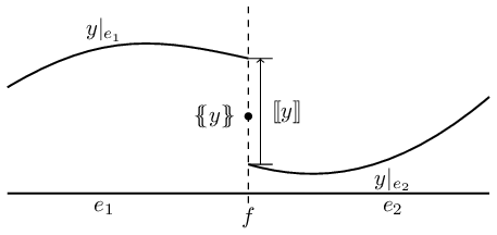
Figure 19 Definition of the average and jump notations, see [Ern and Di Pietro, 2012]

SIP DG Method for the Poisson Problem

First, let us present the SIP DG formulation for the Poisson equation, see [Ern and Di Pietro, 2012] for more details.

Mathematical formulation:

We aim to find \(u \in H^1_0(\Omega)\) such that:

\[-\text{div}(k \nabla u) = HS \quad \Rightarrow \quad a_{dg}(u_h, v_h) = \int_\Omega HS v_h, \quad \forall v_h \in X_{DG}\]

Discrete bilinear form:

Defining \(N_{e_n}\) the number of neighbour elements of an element \(e\) and \(e_n^i\) with \(i \in [0,N_{e_n}]\) the neighbour elements of \(e\) with the convention \(e_n^0 = e\), we introduce the discrete bilinear form:

\begin{align} a_{dg}(u_h, v_h) &= \sum_{\ell=0}^{N_{e_n}} |k|_\ell \int_{e_n^\ell} \nabla u_h \cdot \nabla v_h \\ &\quad - \sum_{f \in F_e} \int_{f} |k|_f \{\{ \nabla u_h \}\}_f \cdot \vec{n}_f [[v_h]] \\ &\quad - \sum_{f \in F_e} \int_{f} |k|_f \{\{ \nabla v_h \}\}_f \cdot \vec{n}_f [[u_h]] \\ &\quad + \sum_{f \in F_e} \frac{\eta}{h_e} \int_{f} [[u_h]]_f[[v_h]]_f \end{align}

where \(h_e\) is a geometrical parameter that corresponds to the diameter of the circumscribed circle of \(e\).

• The first term ensures consistency.

• The second and third terms impose symmetry.

• The last term provides stability.

Matrix structure:

The stencil of the SIP DG method is rather small, as only element-wise interactions take place. The global stiffness matrix \(\mathbf{K}\) has therefore a block-structured form reflecting this stencil:

\[\begin{split}\mathbf{K} = \begin{bmatrix} \mathbf{K}_{1,1} & \mathbf{K}_{1,2} & 0 & \cdots & \\ \mathbf{K}_{1,2}^e & \mathbf{K}_{2,2} & \mathbf{K}_{2,3} & \cdots & \mathbf{K}_{2,N_E} \\ 0 & \mathbf{K}_{2,3}^e & \mathbf{K}_{3,3} & \cdots & \\ \vdots & & & \ddots & \\ & \mathbf{K}_{2,N_E}^e & & & \mathbf{K}_{N_E,N_E} \end{bmatrix}\end{split}\]

Example mesh:

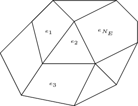
Figure 20 Possible mesh with the Discontinuous Galerkin discretisation

The stability parameter \(\eta\) is not closed by default. A method has been added for automatically computing it in order to ensure coercivity.

Non-Stationary Heat Equation

We now consider the time-dependent heat equation, which models heat transfer in a medium over time.

Problem statement:

For all \(t \in [0, t_{max}]\), find \(T(t) \in H^1_0(\Omega)\) such that:

\[\rho C_p \frac{dT}{dt} - \text{div}(k \nabla T) = HS\]

Physical quantities:

Quantity	Description
\(k\)	Thermal conductivity (W·m⁻¹·K⁻¹)
\(\rho\)	Density (kg·m⁻³)
\(C_p\)	Heat capacity (J·kg⁻¹·K⁻¹)
\(T\)	Temperature (K)
\(HS\)	Heat source (W·m⁻³)

DG Discretization of the Heat Equation

Using a DG formulation, we discretize the heat equation in both space and time.

Weak form:

\[\rho C_p\, m_{dg} \left( \frac{d T_h}{dt}, \theta_h \right) + a_{dg}(T_h, \theta_h) = \int_\Omega f \theta_h, \quad \forall \theta_h \in X_{DG}, \quad \forall t \in [0, t_{max}]\]

The mass bilinear form is defined as:

\[m_{dg}(\tau_h, \theta_h) := \sum_{\ell=1}^{N_{e_n}} \int_{e_n ^\ell} \tau_h \theta_h\]

Time integration methods:

Different schemes are available to advance the solution in time:

• Implicit Euler

  • ✅ Allows for larger time steps

  • ❌ Requires solving a linear system at each time step

• Explicit Euler

  • ✅ Fast, straightforward iterations

  • ❌ Requires small time steps due to stability constraints

DG Options

In your data file, you can add an option DG block as follows

{

order 2 gram_schmidt 1

}

This enables you to secify a custom order of discretisation and the use or not to the Gram-Schmidt orthonormalisation process for your base fucntion. This process is usefull when you work with an explicit scheme as it diagonalise the mass matrix.

For now only order 1 and 2 are available.