Periodic channel flow

This tutorial aims at computing the numerical solution of a 3D incompressible laminar flow with periodic boundary conditions in the Z direction. The geometry is shown in Figure 23 below.

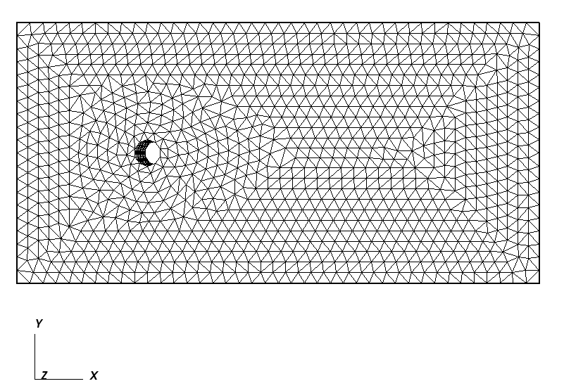
Figure 23 Geometry of the 3D periodic case

Fluid Properties	Value
\(Re\)	2000
\(\rho\)	\(2 kg \cdot m^{-3}\)
\(\mu\)	\(0.01 kg \cdot m^{-1} \cdot s^{-1}\)
Initial velocity \(V0\)	\(1m/s\)

As always when using TRUST, start by loading your TRUST environment, see.

The case we will work with in this tutorial is called P1toP1Bulle in the TRUST repository. It is a 2D simulation of helium gas flow from left to right between two heated walls. Start by copying it into your folder:

source $my_path_to_TRUST_installation/env_TRUST.sh
mkdir -p TRUST_tutorials
cd TRUST_tutorials
trust -copy P1toP1Bulle

Open the P1toP1Bulle.data file and use the RegroupeBord keyword to merge the Entree and Sortie boundaries into a single one named periox.

Then, modify the boundary conditions to apply a periodic boundary condition on the desired boundaries.

Next, change the velocity initial condition to \(U_0=(1,0,0)\).

To speed up the calculation, set the diffusion_implicite option to 1 in the Euler scheme, which makes the diffusive term in the Navier-Stokes equations implicit.

Change nb_pas_dt_max to 30, close your .data file, and run the calculation.

Edit the P1toP1Bulle_pb_Debit.out file and check the flow rate on the periox boundary.

Open the .data file and add the canal_perio source term in the Navier-Stokes equations.

Run the calculation again to check the flow rate evolution over 30 time steps. Also check the pressure and viscous forces applied on the cylinder inside the .out files.

Now, the calculation domain is a channel rotating about the Z axis with a constant angular velocity of \(\Omega=1 rad/s\).

Add the Acceleration source term in the Navier-Stokes equations. Remove the nb_pas_dt_max keyword and set tmax to 100s.

If you wish to practice further, add velocity or statistical post-processing instructions.

Run the calculation.

Afterwards, create a uniformly refined mesh using, for instance, the keyword raffiner_anisotrope.

Then, to improve the calculation speed on this mesh, use the coarser P1 discretization (Read dis { P1 }), which involves fewer pressure unknowns. The calculation should be approximately three times faster than with the P1Bulle discretization, though less accurate: 8452 unknowns compared to 49221 unknowns.

Try another discretization, VEFPreP1B, and re-run the computation by reading the velocity field with the champ_fonc_reprise keyword in the initial conditions for velocity:

vitesse champ_fonc_reprise P1toP1Bulle_pb.xyz pb vitesse last_time

You can also use an implicit scheme to speed up the calculation: switch to the schema_euler_implicite scheme and use an implicite solver. This is only suitable when looking for a stationary state.