PolyMAC_CDO

PolyMAC discretization is based on the development of Compatible Discrete Operators (CDO) schemes. This discretization should make it possible to apply finite volume schemes to non-conforming meshes, with the sole constraint of arranging star-shaped meshes.

Dual Mesh

PolyMAC introduces a rather complex dual mesh. To do so, the gravity center of each control volume \(cv \in \{ E, F, \Sigma, V \}\) corresponding respectively to the cells, the faces, the egdes and the points localization, called \(x_{cv}\) has to be introduce. Then we introduce:

• The dual cell \(\widetilde{v}\) is located at the center of gravity of the cell : \(x_{e}\), see Figure Figure 12.
• The dual face \(\widetilde{\sigma}\) is the line that links the gravity center of the face \(x_f\) to the gravity center of the neighbour cells of the face, see Figure Figure 13.

• The dual edge \(\widetilde{f}\) is the surface that links the gravity center of all of the neighbouring cells \(x_{e}\), the gravity center of all of the neighbouring faces \(x_{f}\) and the gravity center of the edge \(x_{\sigma}\), see Figure Figure 14.

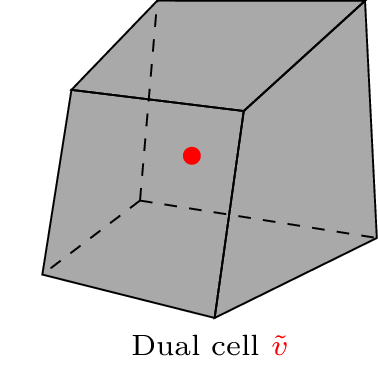
Figure 12 Dual cell when using PolyMAC_CDO

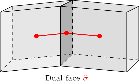
Figure 13 Dual face when using PolyMAC_CDO

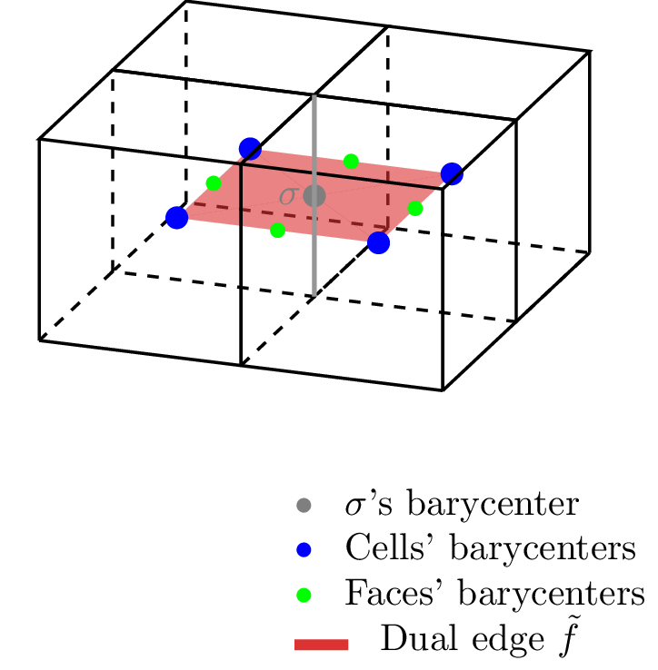
Figure 14 Dual edge when using PolyMAC_CDO

Location of the unknowns

In PolyMAC, unknowns are discretised according to their “physical” properties. A circulation is discretised over an edge, a flux over a face, a potential over the dual cell. Therefore we have:

• The pressure \(p\) is stored at the dual cell: \(p_{\tilde{v}} = p(x_{ev},t)\).

• The normal component of the velocity with respect to a face \(f\) is stored as: \(v_{f} = \frac{1}{|f|} \int u \cdot n dS\).

• The tangential vorticity with respect to an edge \(\sigma\) is stored as: \(\omega_{\sigma} = \frac{1}{|\sigma|} \int \omega \cdot \tau dl\).

CDO scheme

The CDO scheme is based on a set of exact operators that allow you to switch from one location to another on the primal and dual mesh.

Figure Figure 15 summarized the different projection between control volumes in CDO. It is useful to keep it in mind when one want to discretised an equation on a specific control volume.

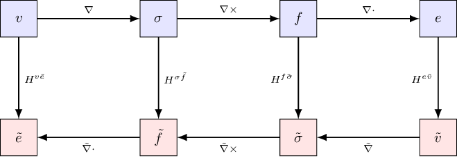
Figure 15 Paths between primal and dual mesh entities and corresponding operators.

Operators can be classified into 2 types:

• The exact operators, such as the gradient or divergence operator, which correspond to linear operators used to move from one discretization to another.

• The approximated operators that introduce approximation error. In particular, Hodge operators are used to establish discrete closure relation linking primal and dual meshes. Other interpolation operators can also be used especially for the convection operator.

Exact discrete operators

Discrete differential operators relies the entities and allow to switch from one localization to another

Exact discrete operator GRAD, DIV and CURL are defined and have their counterpart \(\widetilde{\text{GRAD}}\), \(\widetilde{\text{DIV}}\) and \(\widetilde{\text{CURL}}\) on the dual mesh

Discrete gradient

\[\text{GRAD}:{V} \rightarrow \mathcal{\Sigma}, \hspace{1cm} \forall \sigma \in \Sigma, \forall \mathbf{p} \in V, \hspace{1cm} \text{GRAD}(\mathbf{p})|_{\tilde{\sigma}} = \sum_{\tilde{v} \in V_{\sigma}} \iota_{v,\sigma}p_{v},\]

where \(V_{\sigma} := \{v \in V | v \subset \partial \sigma \}\) and \(\iota_{v,\sigma} = +1\) if \(\tau_{\sigma}\) points towards \(v\), \(\iota_{v,\sigma} = -1\) otherwise

\[\widetilde{\text{GRAD}}:\widetilde{{V}} \rightarrow \widetilde{{\Sigma}}, \hspace{1cm} \forall \tilde{\sigma} \in \widetilde{\mathcal{\Sigma}}, \forall \mathbf{p} \in \widetilde{\mathcal{V}}, \hspace{1cm} \widetilde{\text{GRAD}}(\mathbf{p})|_{\tilde{\sigma}} = \sum_{\tilde{v} \in \widetilde{V}_{\tilde{\sigma}}} \iota_{\tilde{v},\tilde{\sigma}}p_{\tilde{v}}\]

where \(\widetilde{V}_{\tilde{\sigma}} := \{\tilde{v} \in \widetilde{V} | \tilde{v} \subset \partial \tilde{\sigma} \}\) and \(\iota_{\tilde{v},\tilde{\sigma}} = +1\) if \(\tau_{\tilde{\sigma}}\) points towards \(\tilde{v}\), \(\iota_{\tilde{v},\tilde{\sigma}} = -1\) otherwise

Discrete divergence

\[\text{DIV}:F \rightarrow E \hspace{1cm} \forall e \in E, \forall \phi \in F, \hspace{1cm} \text{DIV}(\phi)|_{e} = \sum_{f \in F_{e}} \iota_{f,e}\phi_{f}\]

where \(F_{e} := \{f \in F | f \subset \partial e \}\) and \(\iota_{f,e} = +1\) if \(\nu_{f}\) points outwards \(e\), \(\iota_{f,e} = -1\) otherwise

\[\widetilde{\text{DIV}}:\widetilde{F} \rightarrow \widetilde{E} \hspace{1cm} \forall \tilde{e} \in \widetilde{E}, \forall \phi \in \widetilde{F}, \hspace{1cm} \widetilde{\text{DIV}}(\phi)|_{\tilde{e}} = \sum_{\tilde{f} \in \widetilde{F}_{\tilde{e}}} \iota_{\tilde{f},\tilde{e}}\phi_{\tilde{f}}\]

where \(\widetilde{F}_{\tilde{e}} := \{\tilde{f} \in \widetilde{F} | \tilde{f} \subset \partial \tilde{e} \}\) and \(\iota_{\tilde{f},\tilde{e}} = +1\) if \(\nu_{\tilde{f}}\) points outwards \(\tilde{e}\), \(\iota_{\tilde{f},\tilde{e}} = -1\) otherwise

Discrete curl

\[\text{CURL}: \Sigma \rightarrow F \hspace{1cm} \forall f \in F, \forall \mathbf{u} \in \Sigma, \hspace{1cm} \text{CURL}(\mathbf{u})|_{f} = \sum_{\sigma \in \Sigma_{f}} \iota_{\sigma,f}\mathbf{u}_{\sigma}\]

where \(\Sigma_{f} := \{\sigma \in \Sigma | f \subset \partial f \}\) and \(\iota_{\sigma,f} = +1\) if \(\tau_{\sigma}\) shares the same orientation as the one induced by \(\nu_{f}\), \(\iota_{\sigma,f} = -1\) otherwise

\[\widetilde{\text{CURL}}:\widetilde{\Sigma} \rightarrow \widetilde{F} \hspace{1cm} \forall \tilde{f} \in \widetilde{F}, \forall \mathbf{u} \in \widetilde{\Sigma}, \hspace{1cm} \widetilde{\text{CURL}}(\mathbf{u})|_{\tilde{f}} = \sum_{\tilde{\sigma} \in \widetilde{\Sigma}_{\tilde{f}}} \iota_{\tilde{\sigma},\tilde{f}}\mathbf{u}_{\tilde{\sigma}}\]

where \(\widetilde{\Sigma}_{\tilde{f}} := \{\tilde{\sigma} \in \widetilde{\Sigma} | \tilde{f} \subset \partial \tilde{f} \}\) and \(\iota_{\tilde{\sigma},\tilde{f}} = +1\) if \(\tau_{\tilde{\sigma}}\) shares the same orientation as the one induced by \(\nu_{\tilde{f}}\), \(\iota_{\tilde{\sigma},\tilde{f}} = -1\) otherwise

Hodge operators

Closure relations between the localization in the primal cell and the dual cell are formulated using the construction of non exact global discrete operators called Hodge operators \(H_{\alpha^{-1}}^{\widetilde{\mathcal{X}}\mathcal{Y}}\). They are express using geometric quantities related to the primal and dual mesh entities and some material properties such as diffusivity.

Local Hodge operator must be symmetric, locally stable and \(\mathbb{P}_0\)-consistency

Hodge operators are not unique, the strategy in the CDO scheme consists of defining them using a reconstruction operator \(L_{\mathcal{X}_{e}}\)

\[L_{\mathcal{X}_e}(\mathbf{a})(\overline{x}) := \sum_{x \in X_e} \mathbf{a}_X l_{x,e}(\overline{x}) \quad \forall \mathbf{a} \in \mathcal{X}_e, \forall \overline{x} \in e\]

Orthogonal decomposition of the reconstruction operator into consistent and stabilization parts

\[L_{\mathcal{X}_e} := C_{\mathcal{X}_e} + S_{\mathcal{X}_e}\]

\(C_{\mathcal{X}_e} R_{\mathcal{X}_e} (K) = K\) and \(S_{\mathcal{X}_e} R_{\mathcal{X}_e} (K) = 0\) for constant fields

then the local Hodge operator can be generically defined by:

\[\left.H_{\alpha}^{\mathcal{X}_e\widetilde{\mathcal{Y}}_e}\right|_{x',\tilde{y}(x)} := \int_e l_{x,e}(\overline{x})\alpha l_{x',e}(\overline{x}) \quad \forall x,x' \in X_e\]

We choose here according to description in Bonelle thesis [Bonelle, 2014] (section 7.3.1) and in Codecasa et al. [Codecasa et al., 2010] the Piecewise constant non-conforming reconstruction.

\[L_{\mathcal{X}_e} := C_{\mathcal{X}_e} + \hat{S}_{\mathcal{X}_e}((\mathbb{I}_{\mathcal{X}_e} - R_{\mathcal{X}_e} C_{\mathcal{X}_e}))\]

with \(E_{\mathcal{X}_e} : \mathcal{X}_e \rightarrow \mathbb{P}_0(e)\) and \(\hat{S}_{\mathcal{X}_e} : \mathcal{X}_e \rightarrow \mathbb{P}_0(p_{x,e})\) with \(p_{x,e}\) the partition of the cell associated to the mesh entities \(x\)

Then the local reconstruction of the circulation \(\{\underline{l}_{\sigma,e}\}_{\sigma \in \Sigma_e}\) on the piecewise partition volume \(p_{\sigma',e}, \ \sigma' \in \Sigma_{e}\) corresponding to the subvolume of the cell attached to the edge \(\sigma'\), the center of the cell and the center of the adjacent face (Figure Figure 16). It written:

\[\underline{l}_{\sigma,e}|_{p_{\sigma',e}} = \frac{\beta}{|p_{\sigma,e}|} \underline{\tilde{f}}_e(\sigma) \delta_{\sigma,\sigma'} + \left(\mathbb{I} - \beta \frac{\underline{\tilde{f}}_e(\sigma') \otimes \underline{\sigma'}}{|p_{\sigma',e}|}\right)\frac{\underline{\tilde{f}}(\sigma)}{|e|}\]

Then the local reconstruction of the flux \(\{\underline{l}_{f,e}\}_{f\in F_e}\) on the piecewise partition volume \(p_{f',e}, \ f' \in F_{e}\) corresponding to the subvolume of the cell attached to the face \(f'\), and the center of the cell (Figure Figure 16). It written:

\[\underline{l}_{f,e}|_{p_{f',e}} = \frac{\beta}{|p_{f,e}|} \underline{\tilde{\sigma}}_e(f) \delta_{f,f'} + \left(\mathbb{I} - \beta \frac{\underline{\tilde{\sigma}}_e(f') \otimes \underline{f'}}{|p_{f',e}|}\right)\frac{\underline{\tilde{\sigma}}(f)}{|e|}\]

The choice for the \(\beta\) parameter must be \(\beta = \frac{1}{\text{dim}}\) to yield the DGA reconstruction while the choice \(\beta = \frac{1}{\sqrt{dim}}\) corresponds to the choice made in SUSHI schemes

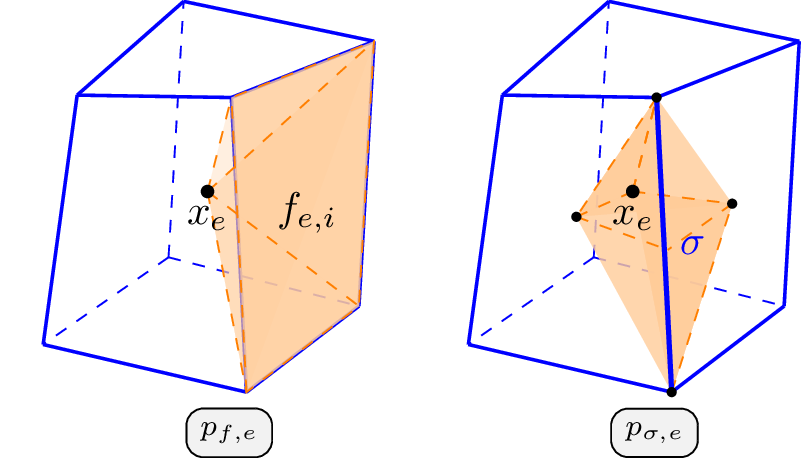
Figure 16 Partitioning of the cell into elementary sub-volumes attached to face \(p_{f,c}\) (left) and to edge \(p_{e,c}\) (right)

Additional reconstruction operator

A first-order reconstruction mapping operator \(\mathbb{R} : F \rightarrow V\) will be used in the convection operator for the Navier-Stokes equations (see Incompressible Navier-Stokes) to interpolate a vector \(\phi\) expressed along the normal of the faces to the center of the cell using the formula (1) from [Basumatary et al., 2014].

(7)\[\phi_\sigma = \frac{1}{|\sigma|}\sum_{f \in \sigma}|f|\phi_f(\vec{x}_f - \vec{x}_{\sigma})\]

Elliptic equations

We first consider here the resolution of a diffusion equation using the CDO schemes

\[-\underline{\nabla} \cdot (\underline{\underline{\kappa}} \ \underline{\nabla} ) = s\]

we introduce the gradient \(\overline{g} = \underline{\text{grad}} \ p\) and the flux \(\overline{\phi} = - \underline{\underline{\kappa}} \ g\)

using cell-based schemes we obtain the discrete system of equations :

\[\begin{split}\begin{cases} \kappa^{-1} \phi + \nabla g = 0 \\ \nabla \cdot \phi = s , \end{cases} \hspace{1cm} \begin{cases} H_{\kappa^{-1}}^{\widetilde{F} \Sigma}(\phi) + \widetilde{GRAD} (p) = 0 \\ DIV ( \phi ) = R_{E}(s) \end{cases}\end{split}\]

with matricial expression

\[\begin{split}\begin{pmatrix} H_{\kappa^{-1}}^{\widetilde{F} \Sigma} & \widetilde{\mathbb{G}} \\ \mathbb{D} & 0 \end{pmatrix} \begin{bmatrix} \phi \\ p \end{bmatrix} = \begin{bmatrix} 0 \\ R_{E}(s) \end{bmatrix}\end{split}\]

with \(\widetilde{\mathbb{G}} = - \mathbb{D}^{T}\)

Stokes equations

The Stokes equations model incompressible flows of viscous fluids where the advective inertial forces are negligible with respect to the viscous forces.

\[\begin{split}\begin{cases} -\underline{\Delta} \underline{u} + \underline{\nabla} p &= \underline{f} \\ \underline{\nabla} \cdot \underline{u} &= 0 \end{cases}\end{split}\]

where \(p\) is the pressure, \(\underline{u}\) the velocity and \(\underline{f}\) the external load.

Bonelle thesis [Bonelle, 2014] chooses to formulated the Stokes equations with the \(\underline{\text{curl}}\) operator using the identity \(-\underline{\Delta} \underline{u} = \underline{\nabla} \times \underline{\nabla} \times \underline{u} - \underline{\nabla} ( \nabla \cdot \underline{u})\)

\[\begin{split}\begin{cases} \underline{\nabla} \times \underline{\nabla} \times \underline{u} + \underline{\nabla} p &= \underline{f} \\ \underline{\nabla} \cdot \underline{u} &= 0 \end{cases}\end{split}\]

using the vorticity \(\underline{\omega} := \underline{\text{curl}} \ \underline{u}\)

\[\begin{split}\begin{cases} -\underline{\omega} + \underline{\nabla} \times \underline{u} &= \underline{0}, \\ \underline{\nabla} \times \underline{\omega} + \underline{\nabla} p &= \underline{f} \\ \underline{\nabla} \cdot \underline{u} &= 0 \end{cases}\end{split}\]

Introducing the mass density \(\rho\) and the viscosity \(\mu\) leads to:

\[\begin{split}\begin{cases} -\mu^{-1}\underline{\omega}^* + \underline{\nabla} \times (\rho^{-1}\underline{\phi}) &= \underline{0}, \\ \rho^{-1}\underline{\nabla} \times \underline{\omega}^* + \underline{\nabla} p^* &= \underline{f}^* \\ \underline{\nabla} \cdot \underline{\phi} &= 0 \end{cases}\end{split}\]

with \(\underline{\phi} = \rho \underline{u}\), \(\underline{\omega}^*=\mu \underline{\omega}\), \(p^* = \rho^{-1}p\) and \(\underline{f}^* = \rho^{-1}\underline{f}\)

We use here two discrete Hodge operators:

\[H_{\rho^{-1}}^{F\widetilde{\Sigma}} : F \rightarrow \widetilde{\Sigma} \hspace{0.5cm} \text{and} \hspace{0.5cm} H_{\mu^{-1}}^{\Sigma\widetilde{F}} : \Sigma \rightarrow \widetilde{F}\]

Then we have the discrete velocity located at dual edges and the discrete vorticity at dual faces.

\[\mathbf{u} = H_{\rho^{-1}}^{F\widetilde{\Sigma}}(\phi) \hspace{0.5cm} \text{and} \hspace{0.5cm} \mathbf{\omega} := H_{\mu^{-1}}^{\Sigma\widetilde{F}} (\mathbf{\omega}^*)\]

we also have the following relation

\[\mathbf{\omega} = \widetilde{CURL}(\mathbf{u})\]

The cell-based pressure scheme is:

Find \((\mathbf{p}^*,\phi,\mathbf{\omega}^*) \in \widetilde{V} \times F \times \Sigma\)

\[\begin{split}\begin{cases} -H_{\mu^{-1}}^{\Sigma\widetilde{F}} (\mathbf{\omega}^*) + \widetilde{CURL} \cdot H_{\rho^{-1}}^{F\widetilde{\Sigma}}(\phi) &= 0_{\widetilde{F}}, \\ H_{\rho^{-1}}^{F\widetilde{\Sigma}} \cdot CURL(\mathbf{\omega}^*) + \widetilde{GRAD}(\mathbf{p}^*) &= S(\rho,\underline{f}^*), \\ -DIV(\phi) &= 0_{E}. \end{cases}\end{split}\]

with matricial expression

\[\begin{split}\begin{pmatrix} -H_{\mu^{-1}}^{\Sigma\widetilde{F}} & \widetilde{\mathbb{C}} \cdot H_{\rho^{-1}}^{F\widetilde{\Sigma}} & 0 \\ H_{\rho^{-1}}^{F\widetilde{\Sigma}} \cdot \mathbb{C} & 0 & \widetilde{\mathbb{G}} \\ 0 & - \mathbb{D}& 0 \end{pmatrix} \begin{bmatrix} \mathbf{\omega}^* \\ \phi \\ \mathbf{p}^* \end{bmatrix} = \begin{bmatrix} 0 \\ S(\rho,\underline{f}^*) \\ 0 \end{bmatrix}\end{split}\]

with \(\widetilde{\mathbb{G}} = - \mathbb{D}^{T}\) and \(\widetilde{\mathbb{C}} \cdot H_{\rho^{-1}}^{F\widetilde{\Sigma}} = H_{\rho^{-1}}^{F\widetilde{\Sigma}} \cdot \mathbb{C}\)

Incompressible Navier-Stokes

\[\begin{split}\begin{cases} \partial_t \underline{u} + \nabla \cdot ( u\otimes u) + \nu \underline{\Delta}(\underline{u}) + \underline{\nabla} p &= \underline{f} \\ \underline{\nabla} \cdot \underline{u} &= 0 \end{cases}\end{split}\]

where \(p\) is the pressure, \(\underline{u}\) the velocity and \(\underline{f}\) the external load.

Using the identity \(-\nu \underline{\Delta} = \nu \underline{\nabla} \times \underline{\nabla} \times \underline{u} - \underline{\nabla} ( \nabla \cdot \underline{u})\) we obtain

\[\begin{split}\begin{cases} \partial_t \underline{u} + \underline{\nabla} \times \underline{\nabla} \times \underline{u} + \underline{\nabla} \cdot (\underline{u} \otimes \underline{u}) + \underline{\nabla} p &= \underline{f} \\ \underline{\nabla} \cdot \underline{u} &= 0 \end{cases}\end{split}\]

using the vorticity \(\underline{\omega} := \underline{\text{curl}} \ \underline{u}\)

\[\begin{split}\begin{cases} -\underline{\omega} + \underline{\nabla} \times \underline{u} &= \underline{0}, \\ \partial_t \underline{u} + \underline{\nabla} \times \underline{\omega} + \nabla \cdot ( u\otimes u) + \underline{\nabla} p &= \underline{f} \\ \underline{\nabla} \cdot \underline{u} &= 0 \end{cases}\end{split}\]

Introducing the mass density \(\rho\) and the viscosity \(\mu\) leads to:

\[\begin{split}\begin{cases} -\mu^{-1} \underline{\omega}^{*} + \underline{\nabla} \times (\rho^{-1}\underline{\phi}) &= \underline{0}, \\ \partial_t (\rho^{-1} \underline{\phi}) + \nabla \cdot \left( (\rho^{-1} \phi) \otimes (\rho^{-1}\phi) \right) + \rho^{-1} \underline{\nabla} \times \underline{\omega}^{*} + \underline{\nabla} p^{*} &= \underline{f}^{*} \\ \underline{\nabla} \cdot \underline{\phi} &= 0 \end{cases}\end{split}\]

The cell-based pressure scheme is:

Find \((\mathbf{p}^*,\phi,\mathbf{\omega}^*) \in \widetilde{\mathcal{V}} \times F \times \Sigma\)

\[\begin{split}\begin{cases} -H_{\mu^{-1}}^{\Sigma\widetilde{F}} (\mathbf{\omega}^*) + \widetilde{CURL} \cdot H_{\rho^{-1}}^{F\widetilde{\Sigma}}(\phi) &= 0_{\widetilde{F}}, \\ H_{\rho^{-1}}^{F\widetilde{\Sigma}} \cdot CURL(\mathbf{\omega}^*) + \partial_t H_{\rho^{-1}}^{F\widetilde{\Sigma}}(\phi) + CONV(\phi) \phi + \widetilde{GRAD}(\mathbf{p}^*) &= S(\rho,\underline{f}^*), \\ -DIV(\phi) &= 0_{E}. \end{cases}\end{split}\]

with matricial expression

\[\begin{split}\begin{pmatrix} -H_{\mu^{-1}}^{\Sigma\widetilde{F}} & \widetilde{\mathbb{C}} \cdot H_{\rho^{-1}}^{F\widetilde{\Sigma}} & 0 \\ H_{\rho^{-1}}^{F\widetilde{\Sigma}} \cdot \mathbb{C} & H_{\rho^{-1}}^{F\widetilde{\Sigma}} \partial_t + \mathbb{T}(\phi) & \widetilde{\mathbb{G}} \\ 0 & - \mathbb{D}& 0 \end{pmatrix} \begin{bmatrix} \mathbf{\omega}^* \\ \phi \\ \mathbf{p}^* \end{bmatrix} = \begin{bmatrix} 0 \\ S(\rho,\underline{f}^*) \\ 0 \end{bmatrix}\end{split}\]

with \(\widetilde{\mathbb{G}} = - \mathbb{D}^{T}\) and \(\widetilde{\mathbb{C}} \cdot H_{\rho^{-1}}^{F\widetilde{\Sigma}} = H_{\rho^{-1}}^{F\widetilde{\Sigma}} \cdot \mathbb{C}\)

The non linear convection term \(CONV\) described in [Beltman et al., 2018] is computing on the using the reconstruction operator (7)

\[\begin{split}\begin{aligned} {[\nabla \cdot ( u\otimes u)]}_{\widetilde{v}} &= \frac{1}{|e|} \sum _{f \in F_e} |f| [{u} \otimes {u}]_f \\ &\simeq \frac{1}{|e|} \sum _{f \in F_e} |f| [u]_f \left( \alpha \left( \gamma [u]_{e_{up}} + \left(1-\gamma \right) [u]_{e_{down}} \right) \right. \notag \\ & \quad \left. + (1-\alpha) \left( \frac{[u]_{e_{up}} +[u]_{e_{down}}}{2} \right) \right), \end{aligned}\end{split}\]

with \(\alpha \in [0,1]\) and \(\gamma \in \{0,1\}\) such that \(\gamma =1\) if \([u_f]\geq 0\) and \(0\) otherwise.

This convective terms must be localized on the dual face:

\[{[\nabla \cdot (u\otimes u)]}_{\tilde{f}} = \lambda_{e,f} [\nabla \cdot (u \otimes u)]_{e} + \lambda_{e',f} [\nabla \cdot (u \otimes u)]_{e'}\]

with the penalty coefficient \(\lambda_{e,f} = \frac{ |\vec{x}_{e' \rightarrow f}|}{|\vec{x}_{e' \rightarrow f}| + |\vec{x}_{e \rightarrow f}|}\) and \(e'\) the neighbouring cell of \(e\) sharing the face \(f\).